FlashAttention-4 from Scratch to Near-SOTA in 60 Diagrams (CUDA/PTX)
Build and understand one of the most complex GPU kernels on the latest hardware
60 diagrams · 14-kernel progression · 94.4% of FlashAttention-4 · CUDA/PTX · video-generation capstone
Contents Open Hide
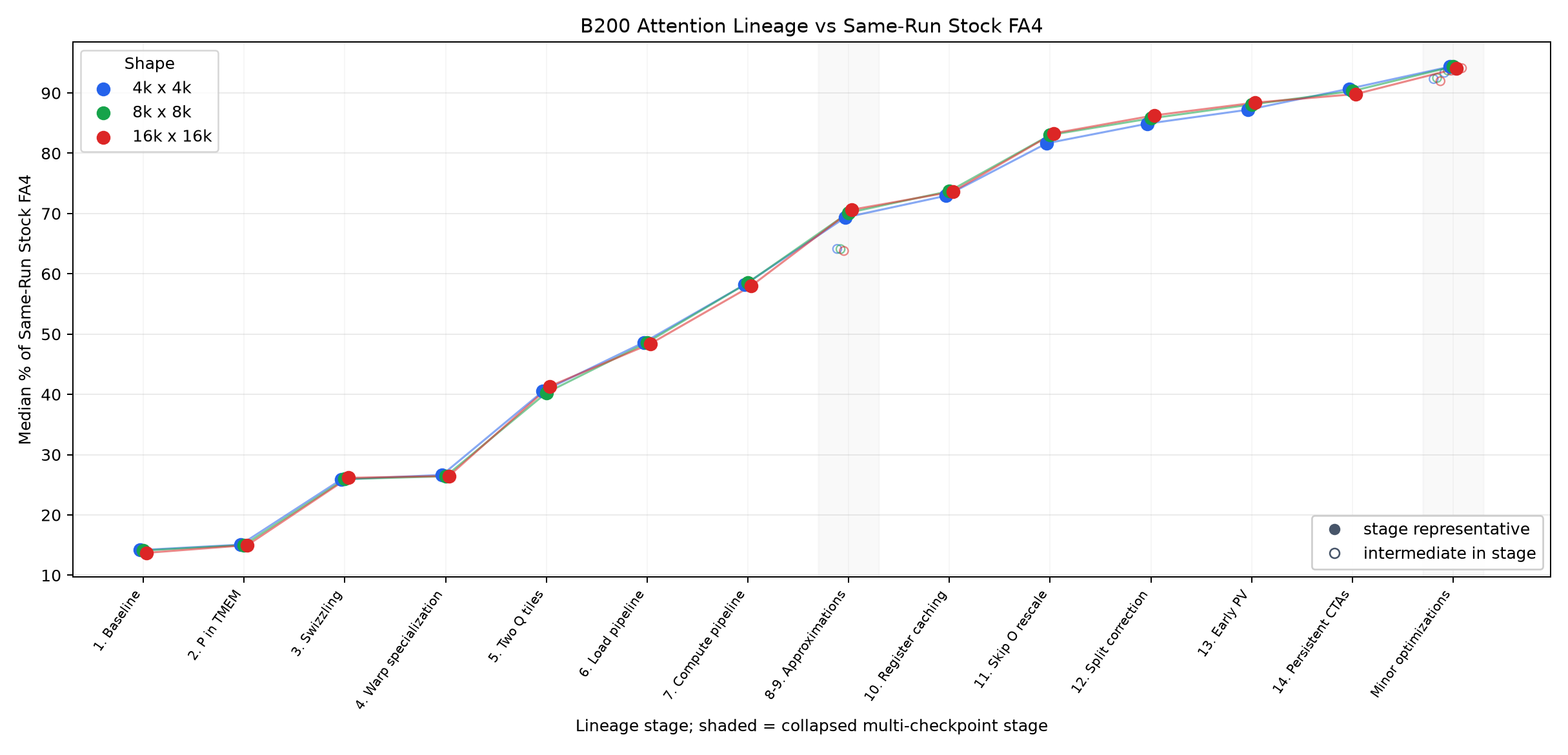
Percent of same-run Stock FA4 across 14-kernel progression and minor optimizations covered at the end. Each implementation is timed on its preferred contiguous layout; see Benchmark Calibration.
What this blog is about
In this blog, we build a dense B200 attention kernel from scratch in CUDA and a little PTX, from baseline to 94.4% of FlashAttention-4 performance on 4K, 8K, and 16K shapes used in the FA4 paper.
The main contribution is the visual guide: a beginner-friendly progression built around 60 diagrams. We first build an intuitive understanding of how the naive kernel works, then add one optimization at a time, with detailed diagrams, concise explanations, and code.
For the capstone project, we plug the final kernel into a video-generation model.
The focus here is not squeezing every last percent of performance, that’ll be the focus of my next blog.
It’s one of the hardest kernels out there, running on the latest hardware, so it’ll be fun.
Research: This is meant to give you a foundation for doing your own GPU kernel research on the latest hardware. We focus on B200 attention, but many of the concepts and mental models apply beyond this kernel. By the end, you’ll understand this kernel and be able to come up with your own optimization ideas.
Prerequisites: I included a beginner on-ramp. If you are a complete beginner, or feel your CUDA foundations are shaky, follow this footnote1 before continuing. I still assume basic CUDA familiarity, but no prior knowledge of Blackwell. New concepts are introduced visually, one piece at a time, and only when they become necessary. So if Blackwell is new to you, just read on. You should be able to follow the progression.
I assume you know what attention is. I also assume some familiarity with ideas behind online-softmax. This part is not Blackwell specific, and there are plenty resources on it.
You do not need to have a B200 at home to follow along, I don’t have one either.
Code: All code is available in my B200 Attention repo. After the baseline, each chapter adds one main optimization. The source code is organized so neighboring kernels are mostly easy to diff. So you can see what each optimization changes, one at a time.
Capstone: At the end, we will plug the kernel you understand into a video-generation model and generate beautiful videos. See the Capstone Project after the main chapters.
DSLs vs CUDA: The original FA4 is written in CuTe, I personally find raw CUDA + a bit PTX simpler to understand (less abstraction layers), so we’re going to implement our kernel in cuda. We will not translate FA4’s CuTe implementation into CUDA syntax, but understand a fast B200 attention kernel in general, through a clean and intuitive progression. Still, FA4 is one of the main references for this work, and most optimization ideas are adapted from it (and FA4 itself is based on cutlass and cute-dsl kernels, see Acknowledgments).
Existing Resources: There are excellent resources explaining optimized matmuls on H200 and B200 (see Acknowledgments). But for B200 attention I haven’t found a deep dive explanation I wanted. Some resources cover the final resulting kernel and don’t explain the progression or lower level motivations behind most optimizations. Others stay high-level and superficial, like summarizing the pipeline and warp roles, but skip most of the work and handholding needed to actually understand the kernel. None gave me the deep explanation I wanted.
Scope: The kernel we gonna be optimizing is dense, head dim 128, non-causal, BF16.
If all you have is AI, we have the same AI as you and are probably better at using it
– tomcr00se
Part I — Basics
Chapter 1 – Baseline Blackwell B200 Attention
i. Roadmap for this chapter
We’ll first study what work each CTA does, and how the work gets assigned to different CTAs of B200 (Work Parallelization section).
Then we’ll take an optional detour for beginners, covering logical vs physical representation, pointers, and tiled matmul.
Then we’ll zoom into our b200 attention kernel and discuss what happens inside each CTA.
All that will be visually explained in much more details later. Just showing the lay of the land for now. Then I will link the code (maps directly to our diagrams).
Baseline attention kernel
Let’s start understanding the first kernel. Our later kernels mostly use
the same math and the same tcgen05 concepts introduced here.
So, in this chapter I’m covering the foundations we’ll use throughout.
That’s why the first chapter is longer than later chapters.
The first kernel exists as a starting point, produces correct numeric results, but not nearly as efficient as our later kernels. This first kernel is already nontrivial and uses many Blackwell-specific features, we will gradually cover them below.
The main bottleneck
Attention is basically two matmuls with a softmax in between. Softmax does far fewer FLOPs, but runs on the ALU and MUFU units, not on tensor cores. And on Blackwell B200, tensor-core throughput roughly doubled while the exp units stayed mostly unchanged (the FA4 paper calls this asymmetric hardware scaling). So at our tile sizes, softmax takes about as many cycles as the very beefy MMAs, so it’s the main bottleneck of this kernel. Most of our optimizations attack this from two sides: making that softmax work cheaper, and overlapping it with the matmuls (ie hiding it in the MMA’s shadow).
ii. Work Parallelization
Before discussing the B200 specific details, let’s first look at how the work is partitioned.
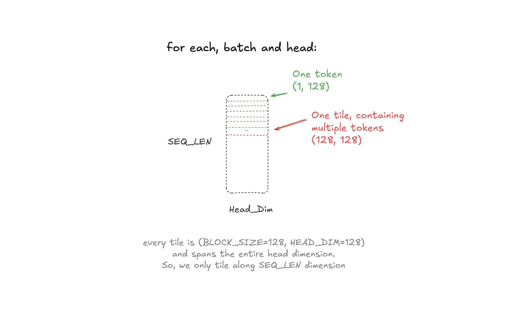
Think of Q, K, V, and the output tensors all having the same shape B, num_heads, seq_len, head_dim.
We split our tensors into tiles, so that they can fit into fast but small on-chip memory.
Our tile sizes are [128, 128], as shown above.
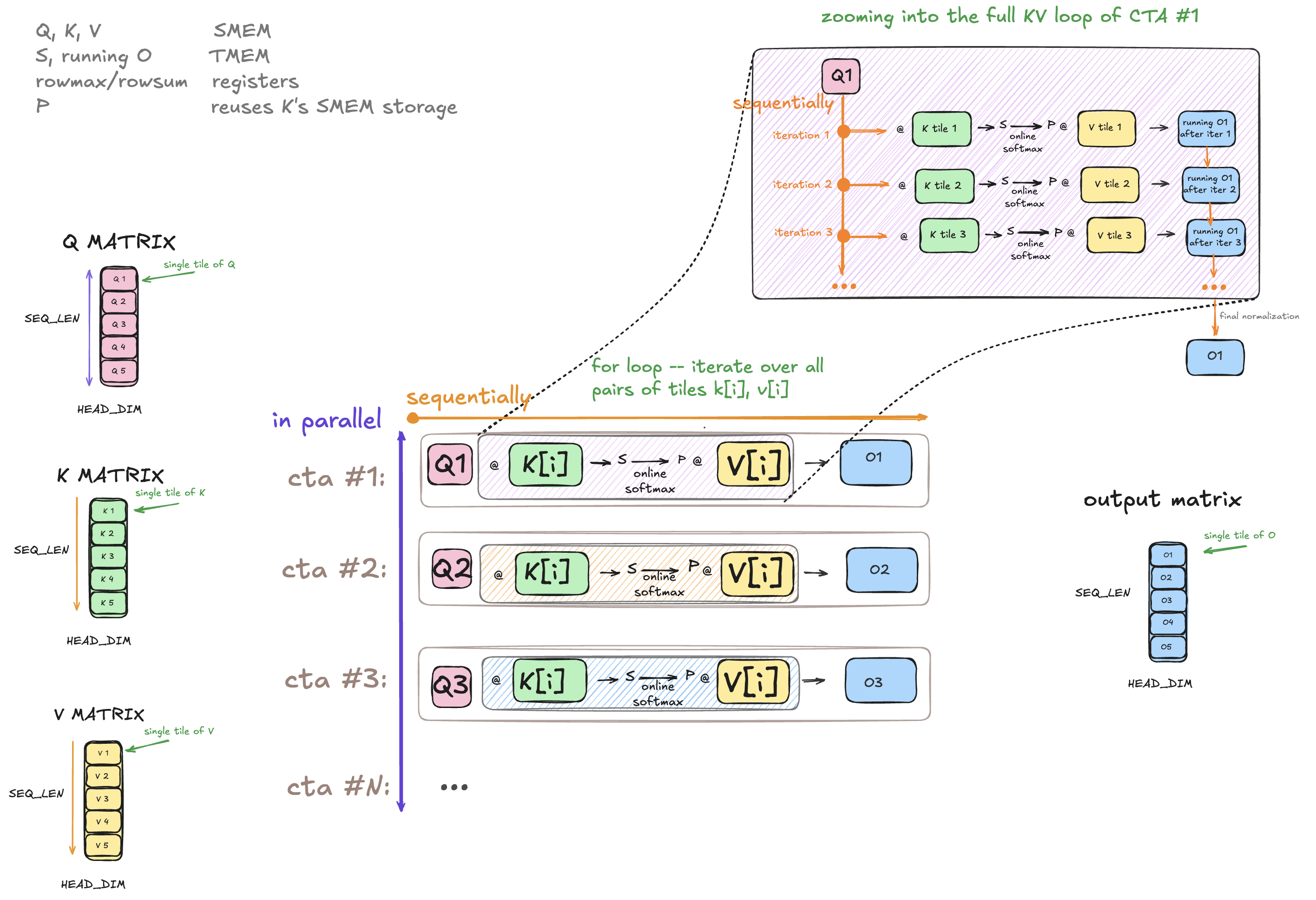
We schedule as many CTAs as there are O (Output) tiles, each CTA produces a single O tile. And collectively all CTAs produce the entire Output tensor (all of its tiles). CTAs execute in parallel (purple arrow).
Within each CTA, the K/V-loop work is sequential (orange arrow).
Let’s zoom into one CTA, as shown above.
To produce its O tile, a CTA loads the corresponding Q tile once, then loops over all K/V tile pairs.
At each iteration of its loop, it computes S_tile = Q_tile @ K_tile.T,
applies online softmax to produce P_tile, and accumulates P_tile @ V_tile into this CTA’s private buffer O-tile.
Inside a CTA, that CTA-private O tile is used as a “running accumulator” (the CTA updates it at each iteration of its K/V loop).
After the final iteration of the K/V loop, CTA normalizes its O-accumulator and stores this completed output tile to global memory.
Don’t worry if some of this doesn’t make sense yet, I’ll explain each step in detail below.
Basically, this split is similar to tiled matmul: different CTAs produce different output tiles, while the loop for one output tile stays inside its CTA. But unlike matmul, attention additionally carries online-softmax state across that K/V loop.
In pseudocode, the high-level flow looks like this:
| |
The outer loop over Q tiles becomes the CUDA grid. The inner loop over KV tiles remains inside each CTA.
Sections labeled in the pseudocode above map directly to B200 code of our first kernel, and will be addressed in detail in this chapter:
- Section A)
Scores = Query @ Key.T(tcgen05 in microtiles, K-major layout) - Section B)
Scores -> Probabilities(reading from TMEM) - Section C)
O += Probabilities @ Values(tcgen05 in microtiles, MN-major layout)
iii. Beginner Onramp — Optional
This section is optional. Skip if you’re already familiar with tiled matmul, the concept of memory layouts, distinction between logical and physical view of the data, and how to use pointers to index into memory.
Similarity to tiled matmul:
Let’s first build one basic tiled-matmul intuition which we’ll use later.
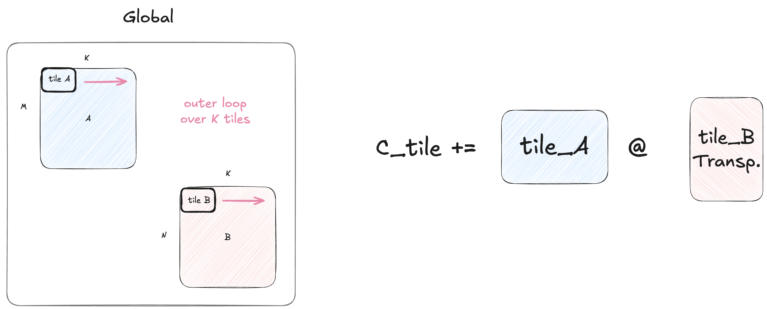
In a regular tiled matmul, we’d split both operand matrices into tiles so that the smaller tiles fit into fast but small on-chip memory, allowing us to reuse each loaded tile multiple times directly from on-chip memory. At each iteration, we’d march along the reduction dim (K, in the diagram), matmul the matching A and B tiles, and accumulate the resulting partials into the same C tile. After processing all K tiles, adding these partials is mathematically equivalent to doing the full matmul without splitting K.
Attention is similar in shape but not exactly:
- generic tiled matmul keeps one C tile fixed and walks along its reduction dimension
- attention keeps one Q tile fixed and walks along the K/V sequence dimension
Introducing layouts:
So we have our tiles of data in global memory.
Suppose we want to matmul a tile of A and a tile of B.
We do not want to implement this matmul in software (by manually looping over individual elements and computing dot products with scalar instructions),
as this will be extremely slow. Instead we want to use tensor cores.
To use tensor cores on Blackwell, we must use the tcgen05.mma family of instructions.
These tile_a and tile_b I visualized above look like 2d matrices,
but of course these are just logical views of the stored data, actual memory is 1d.
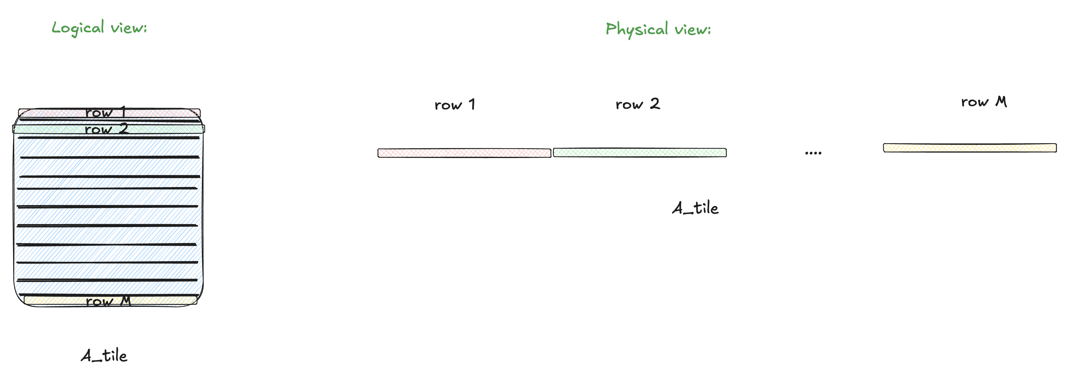
So there’s always some organization of how our data is “laid out” in physical memory.
Let’s say our A operand in GMEM is row-major. In which case physically rows are stored back to back in the 1d memory (shown above).
To find one element in that linear memory, for one [row, col] element, we start from the base pointer and use the strides to compute its offset.
Suppose we have a tiny [2,2] matrix, and we want to get element at my_matrix[1,1].
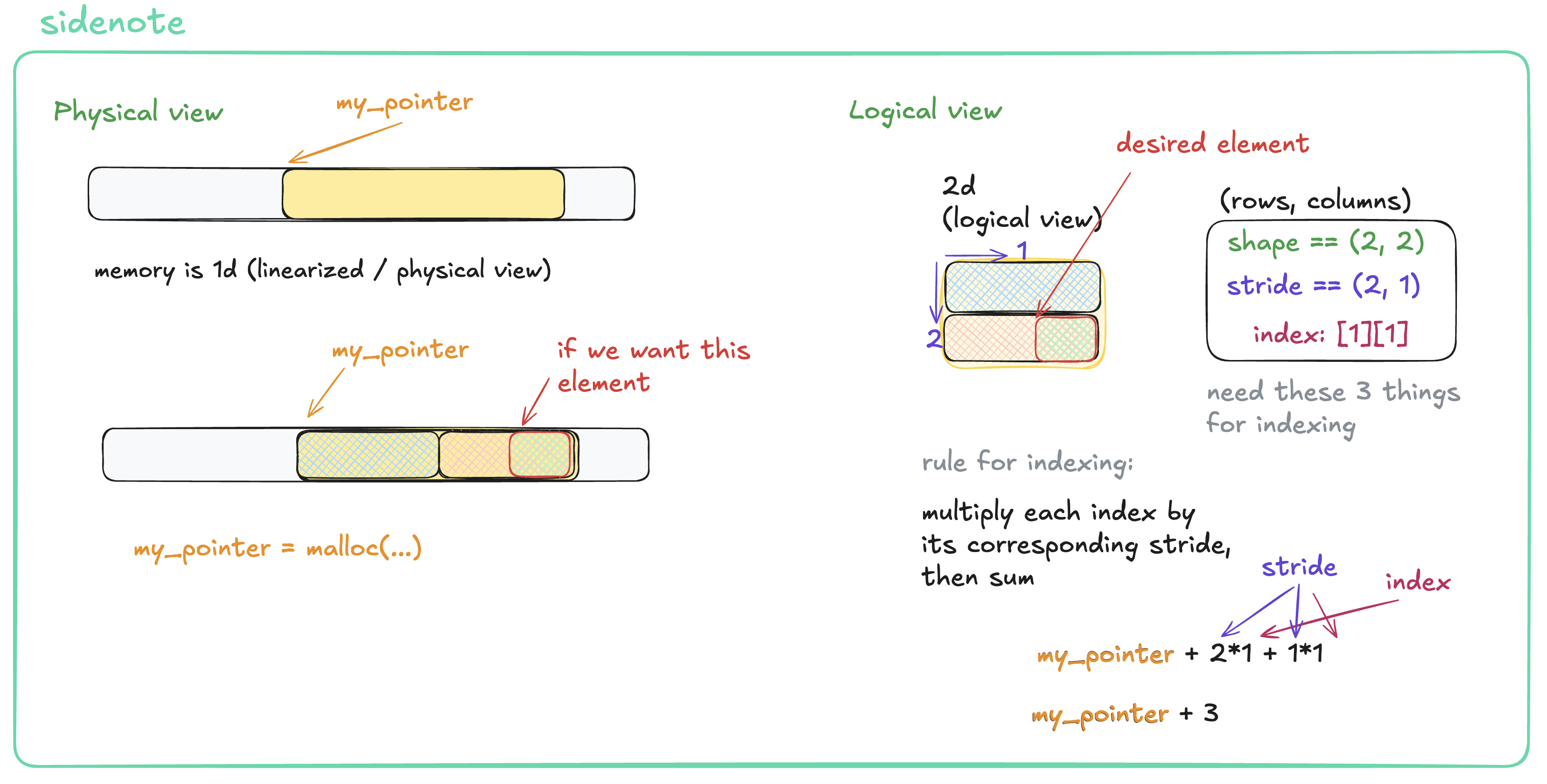
So we have these 2d tiles which are somehow (one way or another) laid out in physical memory.
A layout is the rule that maps logical coordinates, such as [row, col],
to physical memory addresses. Row-major is one such layout.
But, that tcgen05.mma(tile_A, tile_B) which we want to call doesn’t work on
that simple row-major physical layout. It only supports a small number of very specific
layouts (not just plain row-major or col-major; and what specifically
are these layouts expected by the mma is not too important for now, discussed later).
Basically tcgen05 expects data organized in one of specific layouts (ie how the data is laid out in memory). And additionally, tcgen05 does not support using GMEM operands (because GMEM bandwidth is too low, operands need to be written to fast on chip memory first).
The takeaway from this section is, we need to lay out these A and B operands in SMEM, in some certain layout supported by tcgen05.
Back to the main flow (and out of the onramp):
As we saw in the first two diagrams, and the pseudocode, in each CTA, Q stays fixed, while each iteration of the K/V loop computes:
- A)
Q @ K.T -> S - B)
S -> P - C)
P @ V -> O
These are the 3 main computations that each iteration of the KV loop (along the SEQ_LEN) does. Let’s zoom into a single iteration of the K/V loop, and cover these 3 steps one by one.
A) Q@K.T (explaining K-major)
Inside one K/V-loop iteration — Step 1 of 3.
Before running QK, we need Q and the current K tile in SMEM. Q is loaded once for the CTA, while a new K tile is loaded on every K/V iteration. Both Q and K use the same layout, so below I draw only the Q copy and omit the K copy.
Note: In the QK matmul diagrams and code snippets, I use conventional matmul dim names: Q[M,K] @ K[N,K].T = S[M,N]. These are local matmul-axis names, not axis names of our kernel’s input global tensors.
As mentioned earlier, Tensor Cores on Blackwell represented by the tcgen05 family of instructions.
And tcgen05.mma expects its operands be organized in a particular layout
(we cannot just copy our tiles from global to shared in any arbitrary layout and run MMA on that).
Given that constraint, we must “lay out” that data in one of these layouts MMA supports.
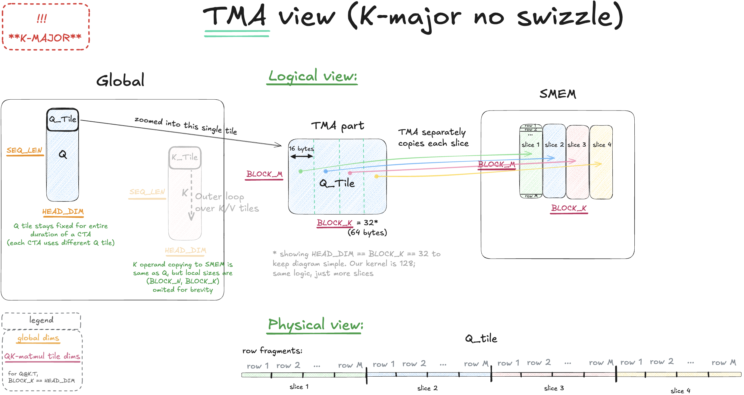
So how specifically we should lay out the data in SMEM, so that it’s one of the layouts supported by MMA? For simplicity, let’s only describe the process of copying Q tile from GMEM to SMEM (the same logic applies separately to the K tile). Logically we’re splitting that Q tile vertically (as shown in the picture – here pictorially 4 slices total). And then copy each slice individually from GMEM to SMEM with TMA2 (see the diagram above).
Why do we need to slice the tile this way instead of copying the whole tile at once? Good question, hold this thought for a moment. I don’t want to introduce too many things at once, so let’s return to this later when it matters. For now just remember we’re copying in slices.
After copying all slices, it seems nothing changed going from GMEM to SMEM
(as visualised, we see the same logical [BLOCK_M, BLOCK_K] matrix but now in SMEM instead of GMEM).
But in fact physically, the representation did change. See “Physical view” green annotation in the picture above.
So the resulting data in SMEM is no longer the row-major layout we had in GMEM.
In the physical SMEM layout we now have all rows of one slice,
only then all rows of another slice and so on.
So this is row-major inside each slice, but overall
(the layout of the entire [BLOCK_M, BLOCK_K] in SMEM)
is not merely a simple row-major or column-major.
Rather, this is one of the so called “canonical layouts” that tcgen05.mma supports.
Remember this term, we will see it often.
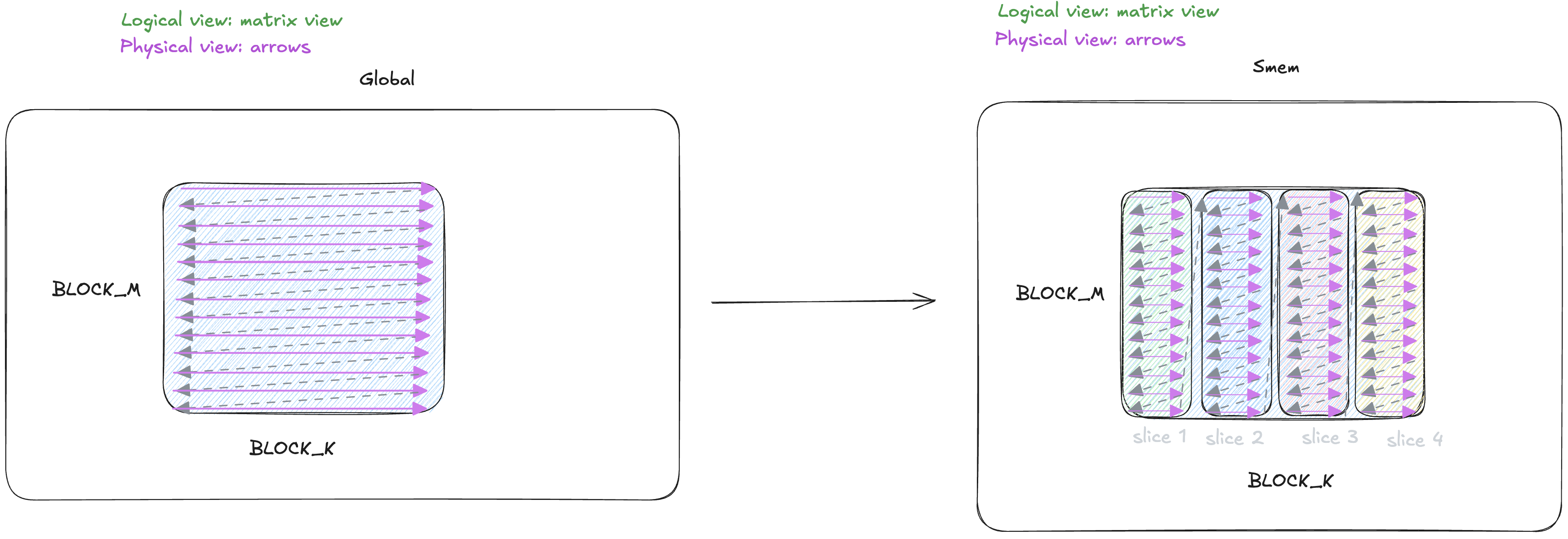
Another visualisation (above) trying to explain differences in the physical representation between the same tile of data (Q tile) in GMEM and in SMEM. Pink arrows denote physical order of elements. GMEM had regular row-major, SMEM has a canonical layout which tcgen05 knows how to work with (this specific layout drawn is so called K-major no-swizzle – we’ll return to this later).
“K” in K-major does not refer to the Key tensor. “K” in K-major means the reduction dimension (in the canonical matmul naming convention), in our case visualized running horizontally across the logical tile. Each vertical slice above covers a small part of that K dimension.
For now can ignore this part, and for simplicity just think of this layout as the only layout tcgen05 supports. Again, I don’t want to introduce too many things at once. We’ll discuss other layouts later when it matters. That’s just to emphasise how the physical organization of the data changed as a result of us copying vertical slices with TMA.
Why physical layout should be this way but not some other arbitrary way? This does seem unintuitive, but I don’t belive there’s a deeper intuition than to say this is one of the canonical layouts tcgen05 supports (according to the nvidia docs). Some things are ultimately a hardware contract we have to fallback on as ground truth.
Here is the copying logic in code, slightly simplified. At each iteration, src_col selects the next eight columns of Q, and dst_smem selects where to place the copied slice in SMEM.
Q_tmap contains metadata telling TMA how to read Q: its global-memory address, dtype, dims, strides, and copy shape – here (BLOCK_M rows, 8 columns) of BF16 values.
TMA uses this metadata together with the source coordinates and SMEM destination pointer to copy the selected slice.
Note we specify the source and destination differently. For Q, we give TMA row and column coordinates, Q_tmap tells it how those coordinates map to global memory. For SMEM, we give it a byte address directly. That’s why src_col counts columns, but the destination offset is measured in bytes.
int SLICE_COLS = 8;
int SLICE_BYTES = (BLOCK_M * SLICE_COLS) * 2;  // each BF16 value is 2 bytes

// one thread issues all copies in this loop
for (int slice = 0; slice < BLOCK_K / SLICE_COLS; ++slice) {
    // move right to the next source slice
    int src_col = slice * SLICE_COLS;               // column idx

    // Q_smem is starting byte address in SMEM,
    // place next slice after the previous one in SMEM
    int dst_smem = Q_smem + slice * SLICE_BYTES;    // byte address

    // TMA copy
    tma::copy_2d_gmem_to_smem(
        dst_smem,            // destination byte address in SMEM
        &Q_tmap,             // Q's metadata (address, dtype, dims, strides, and copy size)
        src_col,            // starting source column (advances by 8 each iter)
        q_row0,              // this Q tile's first global row (stays fixed)
        mbar_addr            // barrier to track copy completion
    );
}
There’s no software loop over rows here, each TMA call copies one complete (BLOCK_M, 8) slice. We advance the SMEM destination by SLICE_BYTES to place each new slice right after the previous one. So in physical memory, we have all rows of slice 0, then all rows of slice 1, and so on. As shown in the diagram above.
Here, BLOCK_K = 128, so this loop issues 16 copies. The simplified diagrams show only 4 slices. Barrier setup and the completion wait are omitted here.
Above we’ve covered the TMA part: copying data from GMEM to SMEM. Now let’s also discuss the MMA part: how can we actually now run MMA on that SMEM data we’ve prepared.
We used TMA to copy data from Global memory into SMEM, but it’s just a copying mechanism and is not inherently aware about the downstream tcgen05.MMA we’re about to call. And separately, tcgen05.MMA knows only how to interpret a small set of specific layouts, and it doesn’t know how the data it’s about to read got into SMEM in the first place. So, we can think of it as: load part (discussed earlier), and MMA part (discussed below). These are two independent steps and are not aware about each other, so it’s our job to make sure they agree on the same layout.
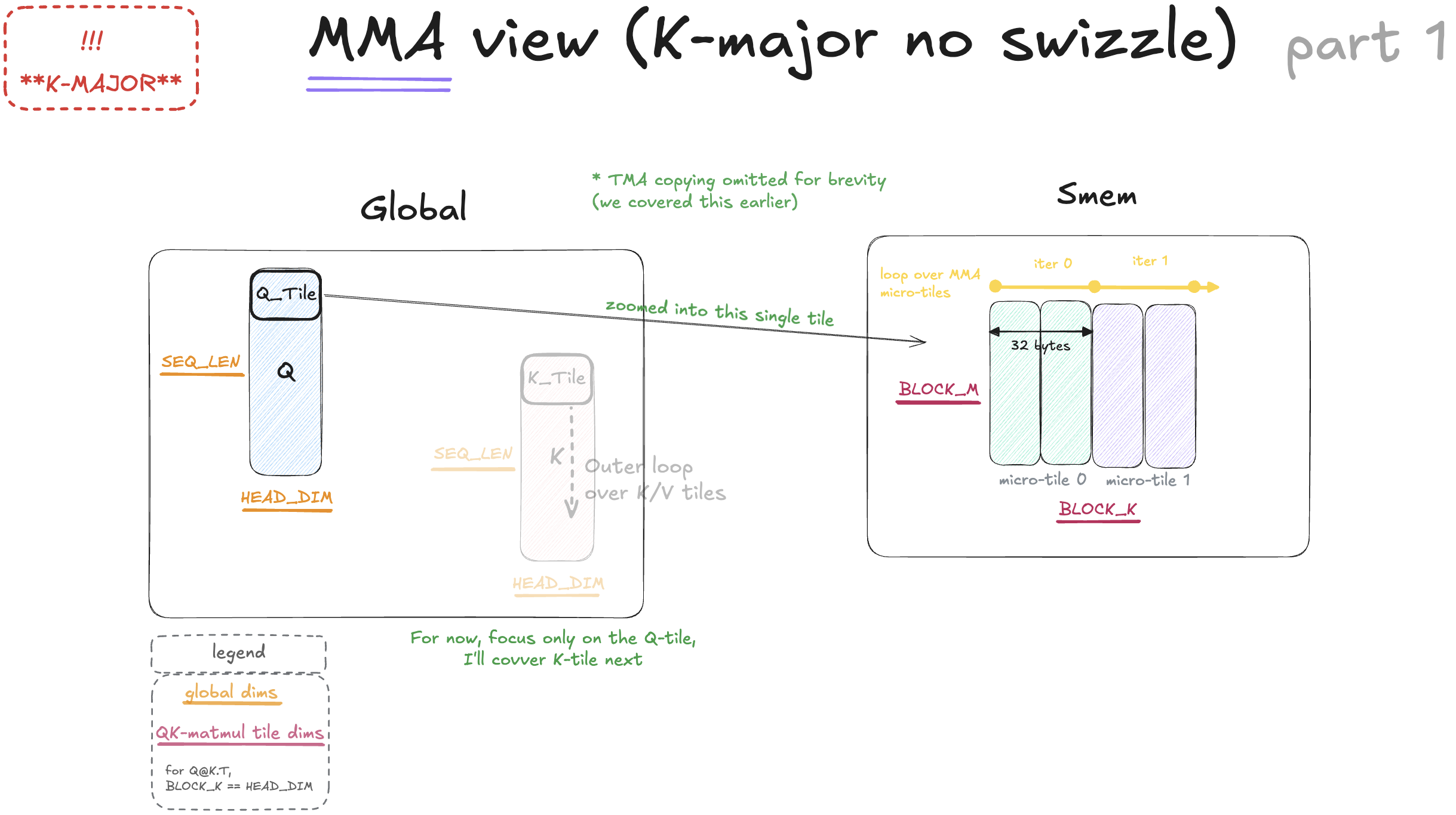
Diagram simplification: diagram uses BLOCK_K = HEAD_DIM = 32 BF16 elements (64B) to keep it readable. The code and the text below use BLOCK_K = HEAD_DIM = 128 BF16 elements (256B). Everything explained below works the same, the actual code just contains 4 times as many slices.
To recap, we earlier copied both of our Q_tile and, separately K_tile into SMEM (in 16B slices along K).
Now we need to take this (block_m, block_k) Q tile, and matmul it with the (block_n, block_k).T K tile.
For now let’s only focus on the Q tile (1st input to the tcgen05.mma), while for now omitting K tile (2nd input to the tcgen05.mma).
Our tiles have BLOCK_K = 128 elements (which is 256 bytes, given our bf16 dtype).
But one tcgen05.mma instruction consumes MMA_K=16 BF16 elements (32B) along K.3
So, the mma_K width is smaller than our tiles K width, thus we need a for loop which walks over the BLOCK_K dim of our Q and K tiles
in steps of 32 bytes (software loop over the data in smem, shown in yellow above).
Each of our Q slices is 16B wide along K, while one tcgen05.mma consumes 32B along K. So two neighboring Q slices form one Q micro-tile. In the diagram above, each same-colored pair of slices forms one micro-tile.
And when I say “micro-tile” I mean a BLOCK_M=128, MMA_K=16 chunk which tcgen05 consumes directly.
A “micro-step” is one tcgen05.mma call consuming one Q micro-tile and one corresponding K micro-tile.
Since BLOCK_K=128 and MMA_K=16, 128 / 16 = 8 micro-steps cover the full reduction-K dimension.
The simplified diagram shows two of those eight steps.
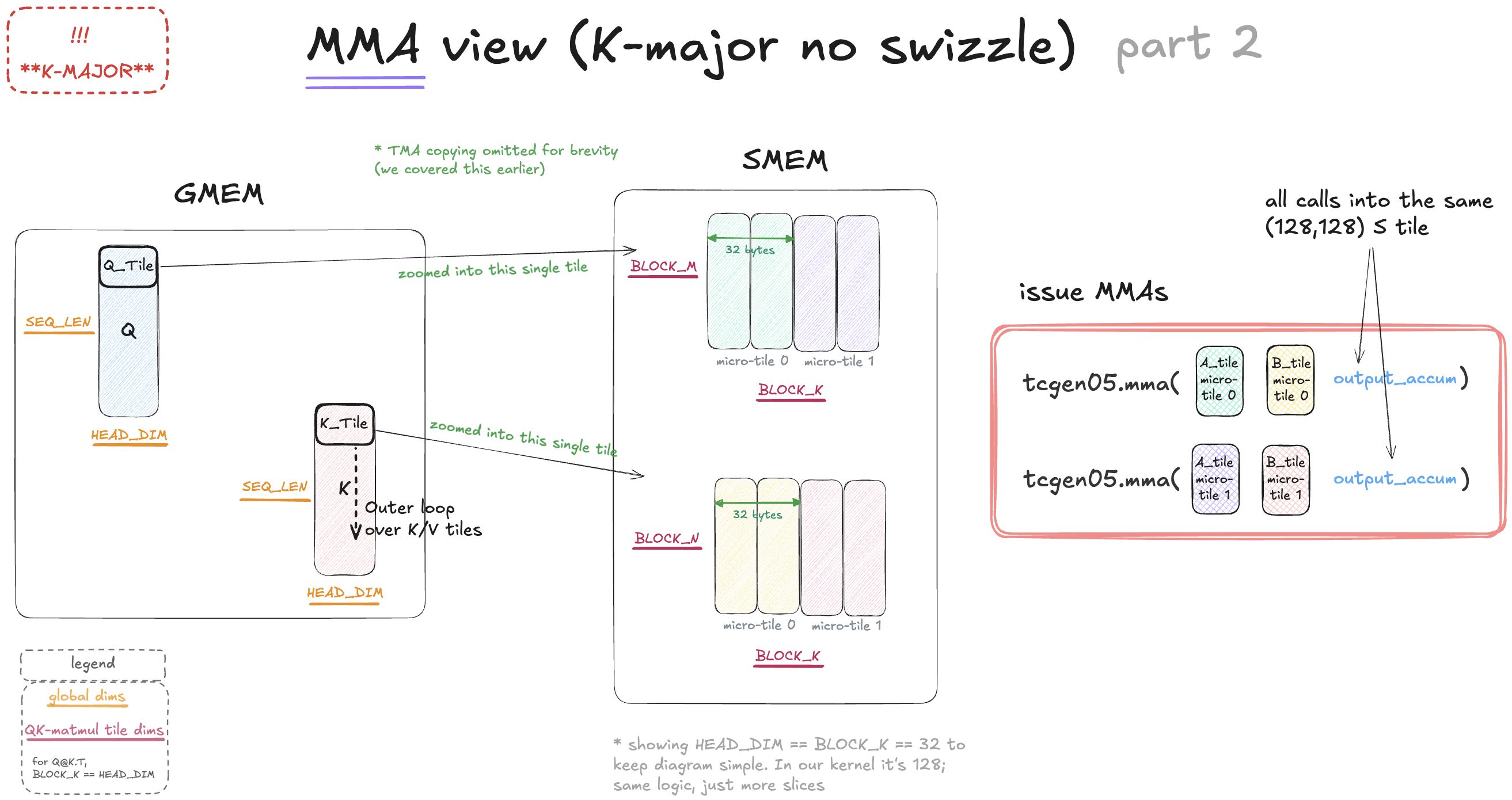
To try to visualise this further, I’ve drawn K_tile as well. Which was independently split on 16B wide slices and copied with TMA, then each pair of its slices is treated as a micro-tile (same as for the Q tile we covered earlier, so I omitted showing copying the K_tile from the diagrams).
Then, to matmul the Q_tile and K_tile tougether, we basically need to matmul their corresponding micro-tiles (shown in the red box in the diagram above):
- 1st Q micro-tile @ 1st K micro-tile.T
- 2nd Q micro-tile @ 2nd K micro-tile.T
The output_accum shown in the picture above is our Scores tile (S).
On Blackwell, tcgen05.mma accumulates its output in Tensor Memory (TMEM),
a dedicated on-chip memory separate from SMEM and registers.
(on earlier GPUs, tensor-core accumulators lived in registers instead).
All QK micro-steps accumulate into the same S tile in TMEM.
For now, just keep in mind that MMA outputs live in TMEM. We’ll explain how
TMEM is allocated and accessed in Section B, when softmax needs to read S.
We turn the above straight-line MMA calls into a loop which iterates over BLOCK_K dim of Q_tile and K_tile using MMA_K=16 micro-steps. In pseudocode:
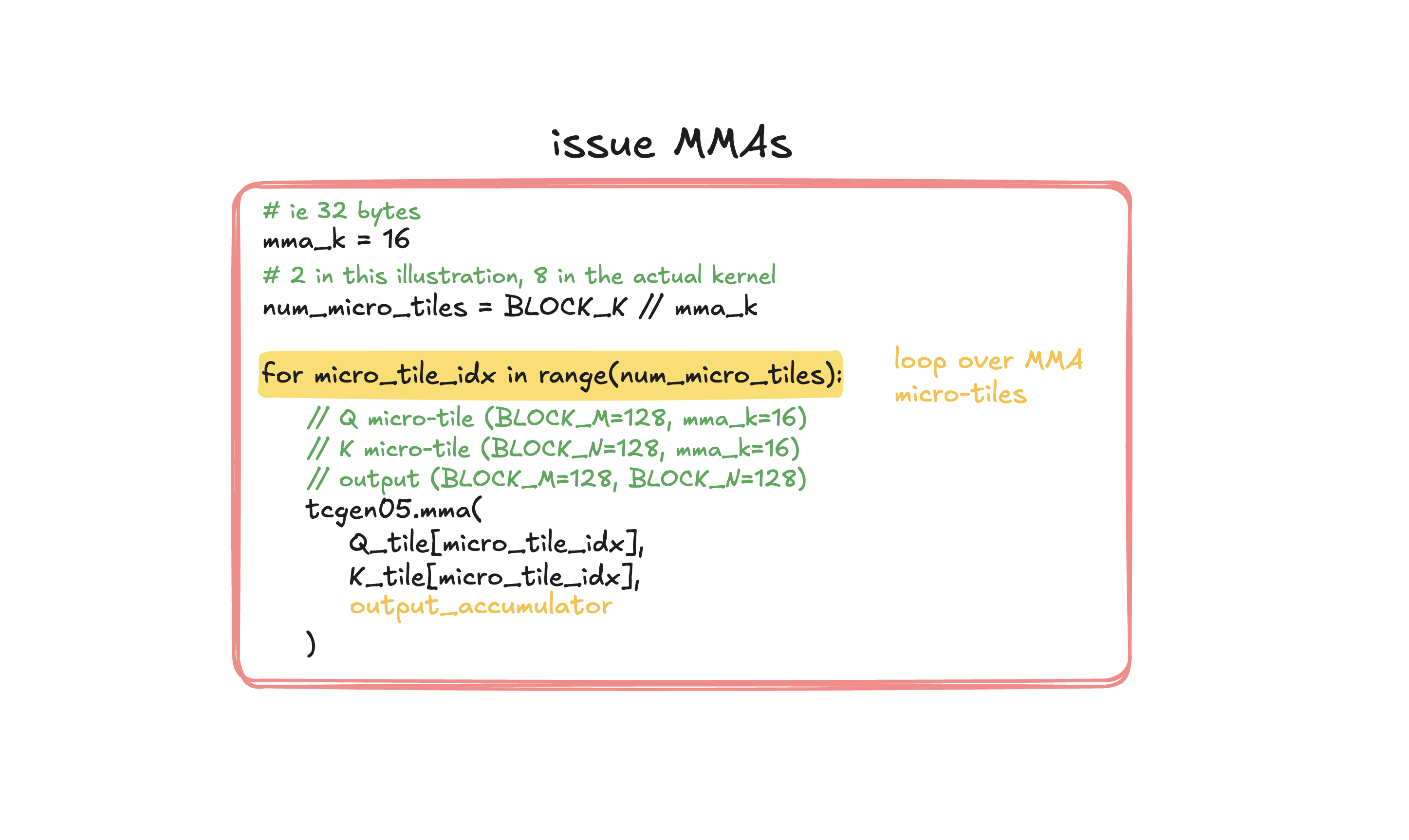
This is our “yellow” loop from the actual kernel code, slightly simplified (executed by a single thread):
// tcgen05 mma_k width along K-dim
int MMA_K_BYTES = 32; // in bytes
int MMA_K = 16; // in BF16 values

// for now, think of each K-major SMEM "descriptor" as a
// pointer-like value selecting current micro-tile
// (it also contains some layout metadata, covered later)
uint64_t q_desc = noswizzle::desc_kmajor(Q_smem, BLOCK_M);
uint64_t k_desc = noswizzle::desc_kmajor(K_smem, BLOCK_N);

// offsets to advance the descriptors to next Q and K micro-tiles
// (minor detail, divide by 16 because descriptor addresses are encoded in 16B units)
uint64_t q_desc_step = (BLOCK_M * MMA_K_BYTES) / 16;
uint64_t k_desc_step = (BLOCK_N * MMA_K_BYTES) / 16;

// BLOCK_K = 128, MMA_K = 16, so 8 micro-steps
for (int k = 0; k < BLOCK_K / MMA_K; ++k) {

    // one micro-step
    tcgen05::mma_f16(
        taddr_s, q_desc, k_desc,
        /*MMA shape and dtypes=*/i_desc_qk,
        /*enable_input_d=*/(k == 0 ? 0 : 1));

    // advance descriptors to the next pair of micro-tiles
    q_desc += q_desc_step;
    k_desc += k_desc_step;
}

// make mbarrier track completion of all 8 micro-steps
tcgen05::commit_arrive(mbar_addr);
// the wait and required synchronization are omitted here
Each iteration calls tcgen05.mma on the next MMA_K=16 chunk and accumulates into the same S tile. First MMA micro-step initializes S, remaining seven MMA micro-steps accumulate into that same S tile. After the loop over all micro-tiles and the completion wait, that S_tile contains the result of Q_tile @ K_tile.T.
No explicit K_tile transpose is needed. Both Q and K use K-major layouts. The MMA A operand reads Q[m,k] directly. For the B operand, tcgen05.mma interprets the stored K tile as the [k,n] operand required for Q @ K.T. K-major itself does not mean “transpose this operand”: A and B are different MMA operand slots with different logical shapes, [M,K] and [K,N], and are therefore interpreted differently by MMA.
We’ve now seen the QK micro-step loop in code. There, we treated q_desc and k_desc as pointer-like values selecting the current micro-tiles. Now let’s unpack the layout information these descriptors also contain, and how MMA uses it to find the data inside each micro-tile.
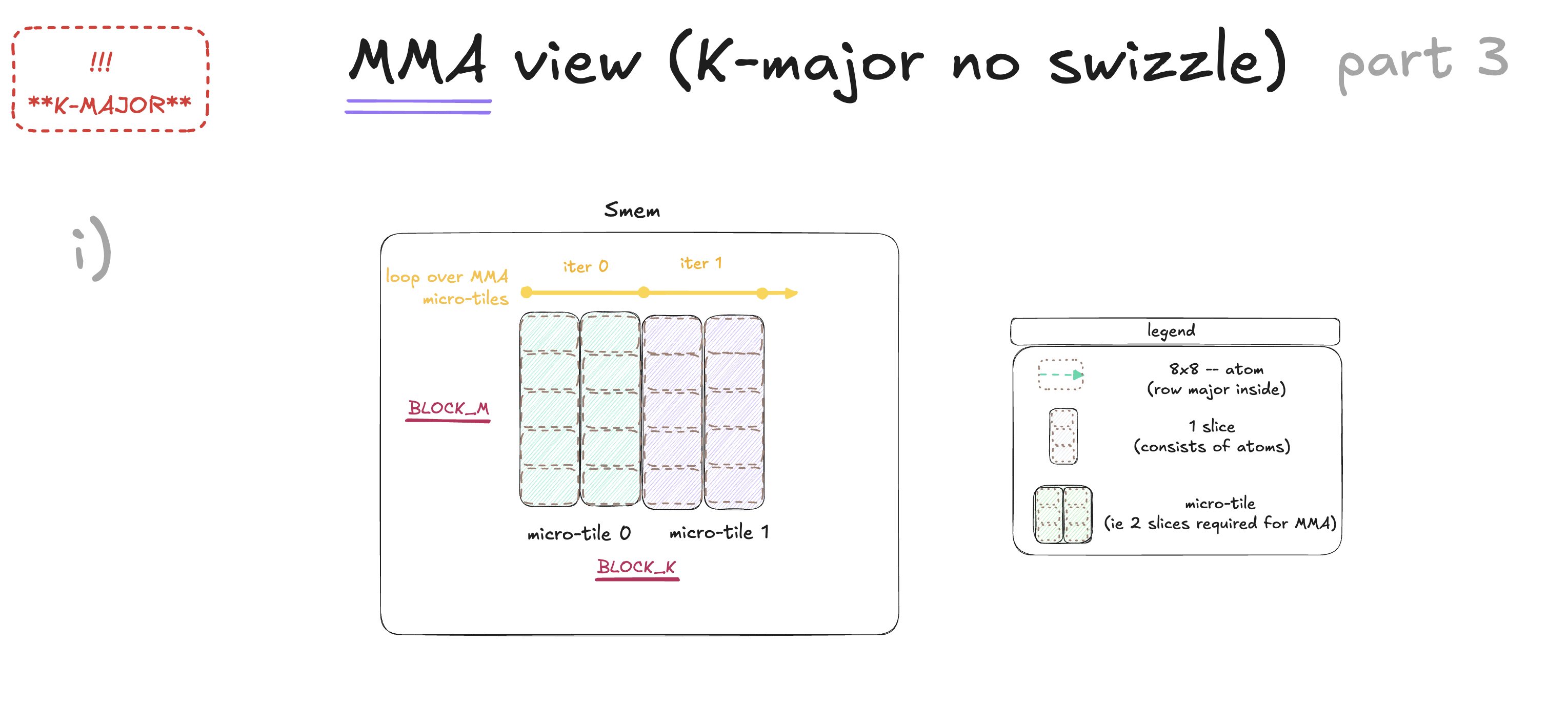
Turns out, there’s one more level of granularity here. Let’s zoom on a Q micro-tile (BLOCK_M=128, MMA_K=16), though the same logic applies to K micro-tile as well.
These micro-tiles themselves consist of lower level units. Called atoms (or “swizzle atoms” as per the cuda docs, note we are NOT doing any swizzling yet, NVIDIA uses “swizzle layout atom” as the umbrella term even when the swizzling mode is None (table 53)).
The size of these atoms depends on the specific canonical layout we’re using, and in our case (the layout we’re using is called K-major no swizzle, but for now we can ignore these details and assume there’s only a single layout that tcgn05.mma supports), these atoms are (8, 8).4
The top-down story so far (see legend in the diagram above): a micro-tile consists of 2 slices, each of which consists of atoms. We need to understand how atoms are arranged in SMEM. But they are not independently programmable MMA units. When issuing MMA we’re still operating on the level of micro-tiles, not individual atoms.
Now we can answer the question from earlier: why did we copy Q and K with TMA in 8-element-wide vertical slices instead of copying the whole tiles at once?
The slice width we used earlier wasn’t arbitrary: it was actually one atom wide. For Q, each (128,8) slice we used, is a vertical stack of (8,8) atoms. So we split the tile into these slices and use TMA to copy one complete stack at a time, placing the stacks one after another in SMEM. This produces the K-major physical atom order that tcgen05.mma supports.
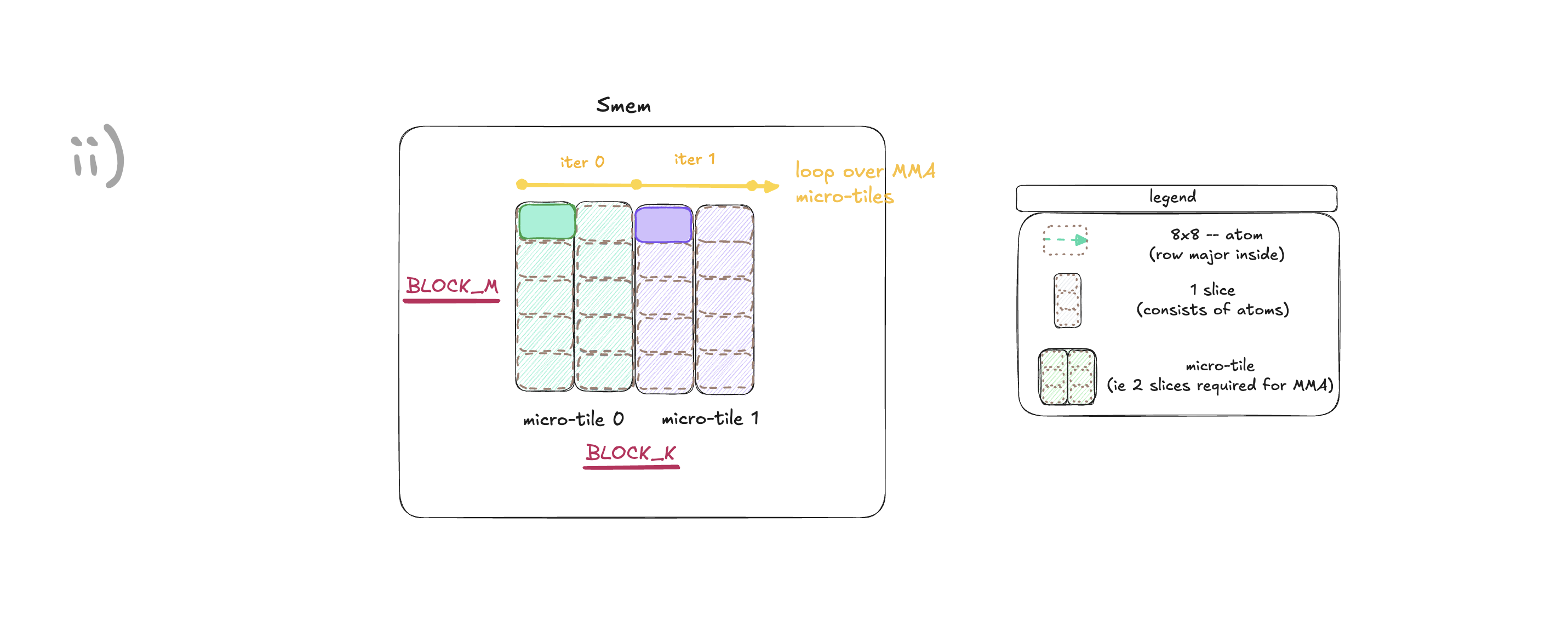
Remeber as discussed above, at each iteration of the “yellow” loop we feed to tcgen05.mma two micro-tiles of data (one Q micro-tile and one K-micro tile).
For a single micro-tile we don’t need to provide to mma the addreses of all its atoms. Instead, we need to provide the base pointer to the first atom, highlighted in the picture above.
As the yellow loop progresses, we advance the base pointer from one micro-tile to the next. In the first iteration, it points to cyan atom, the start of micro-tile 0. In the second iteration, it points to purple atom, the start of micro-tile 1, and so on across the K dimension. The same happens for the K operand descriptor.
But becuase the base points only to the first atom, intuitively, in addition to that base address, MMA somehow needs to know how to step from the first atom in a given micro-tile to other atoms in the same micro-tile.
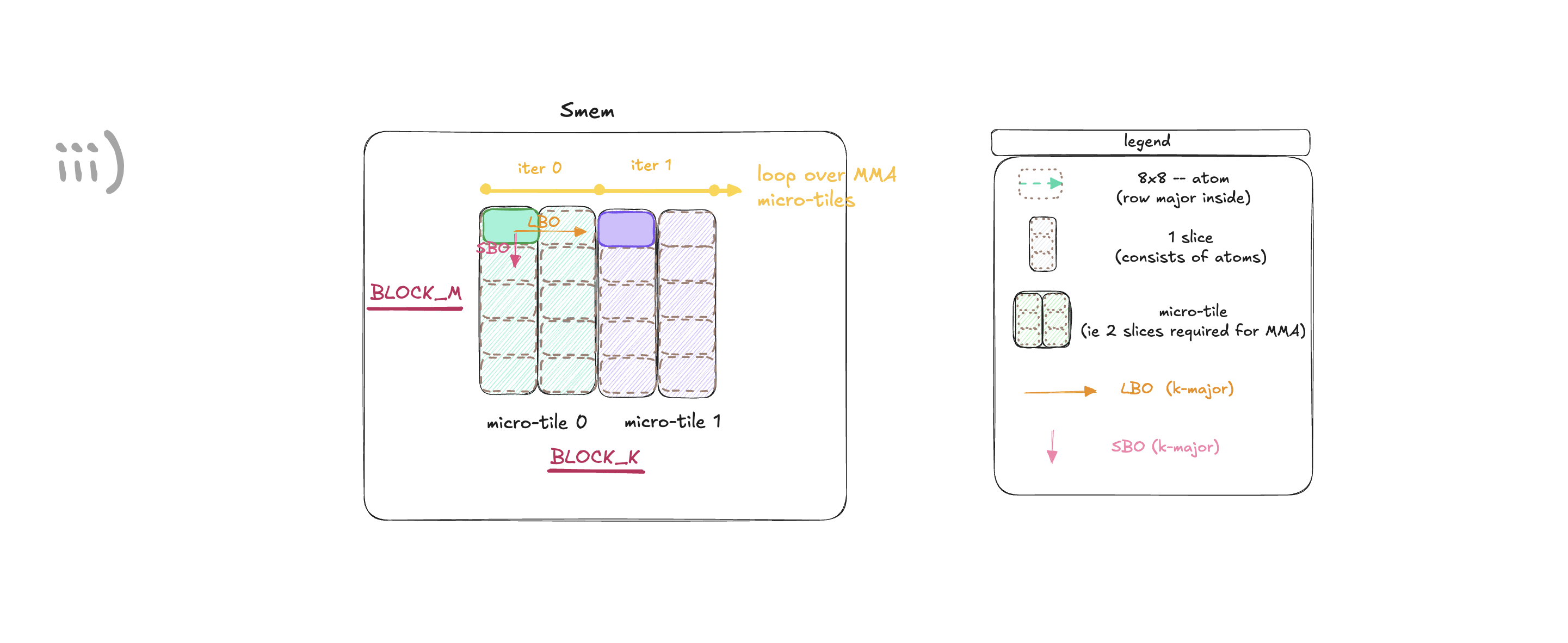
To that end, there’s a concept of SBO and LBO (shown in the figure above). These do not create extra software loop iterations, they describe where the other atoms in the same micro-tile are relative to its base pointer. SBO tells MMA how to step to the next atom in the same slice, and LBO tells MMA how to get to the atom (at the same index) but in the next slice.
In our case, for the SMEM memory layout we’re discussing (k-major no swizzle), each atom, and therefore each vertical slice, is 8 BF16 elements (16B) wide, so:
SBO = 8 rows * 16B per row = 128B   // step over one atom
LBO = BLOCK_M rows * 16B per row = 2048B    // step over one complete slice of atoms
Here, LBO is the same SLICE_BYTES we used in the Q-copy loop, the offset between neighboring vertical slices in SMEM.
Each Q micro-tile contains two slices. So the loop advances the descriptor’s base address by 2 * SLICE_BYTES bytes to reach the next micro-tile.
Descriptor addresses are encoded in 16-byte units, so dividing by 16 gives the q_desc_step used in the code above.
Putting it together, our software loop advances the base pointer from one micro-tile to the next, while SBO and LBO describe the offsets to the other atoms inside the current micro-tile.
B) Online Softmax (explaining S->P)
Inside one K/V-loop iteration — Step 2 of 3.
At this point we finished going through the first matmul (Q@K.T), and now we’re appraoching the online softmax part of our kernel (S –> P).
The online-softmax math is standard and not specific to B200, and there are plenty of explanations elsewhere, so I won’t rederive it here. I’ll only summarize the state update we need, then focus on how our B200 kernel implements it.
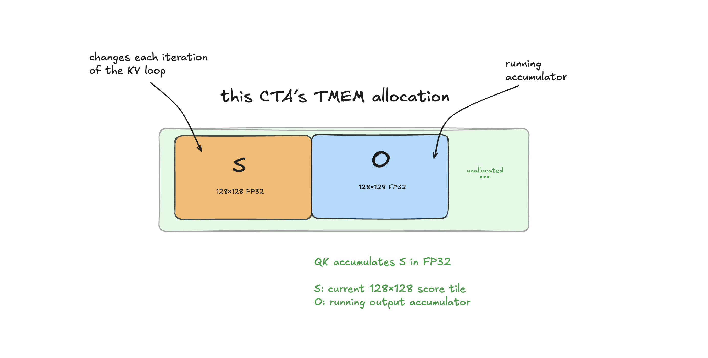
We already briefly saw TMEM in Section A, our Q @ K.T micro-steps accumulated S there. Now let’s zoom in on TMEM itself and see how online softmax reads S and converts it into P.
TMEM is (128 rows, 512 columns), and it must be explicitly allocated. Before the K/V loop, Kernel 1 allocates 128 columns for S and another 128 for O. (allocation is in columns, each column contains 128 elements, so allocating 128 columns allocates a chunk of [128,128] fp32 elements in TMEM).
S holds the current K/V tile’s scores and is overwritten on each iteration of the K/V loop.
O is the running output accumulator, the P@V matmul in the later Section C adds to it on each K/V iteration.
tcgen05.alloc writes the allocation’s base TMEM address into the shared-memory slot tmem_addr.
We then split that allocation into the S and O addresses:
int TMEM_S_COLS = 128;
int TMEM_O_COLS = 128;

__shared__ int tmem_addr[1];

// simplified PTX notation
// warp selection and synchronization omitted.
tcgen05.alloc(tmem_addr, TMEM_S_COLS + TMEM_O_COLS);

// first 128 columns for S, next 128 for O.
int taddr_s = tmem_addr[0];
int taddr_o = taddr_s + TMEM_S_COLS;
Let’s open up this abstraction we saw earlier:
# Section B: S -> P, update rowmax/rowsum, and correct old O
P, softmax_state, O = online_softmax_update(
    S, softmax_state, O
)
For one K/V iteration, the state changes like so (first let’s see it in pseudocode):
// Section A, covered earlier
// S = Q @ K.T;

// Section B:

tile_rowmax = row_max(S);
// new basis
new_rowmax  = max(running_rowmax, tile_rowmax);

// rescale old state to the new basis
rescale     = exp(running_rowmax - new_rowmax);
running_rowsum *= rescale;
O              *= rescale;

// produce P and update denom
P               = exp(S - new_rowmax);
running_rowsum  += row_sum(P);
running_rowmax   = new_rowmax;

// Section C, covered later:
// O += P @ V;
// after complete K/V loop:
// output = O / running_rowsum;
This is generic online softmax update, not B200 specific so I will not dwell on it. Our main question is how to map this to a B200 kernel.
The pseudocode above contains many individual state updates, but in our kernel, all this online-softmax work above is basically organized around 3 passes over TMEM . And all the other state-updates from the pseudocode above are mostly folded into these 3 passes. So, for the online-softmax update think on the granularity of “3 passes over tiles of data stored in TMEM”.
The 3 passes can be grouped as such:
- 2 passes over S tile – used together to produce P, and
- 1 pass over O tile – used to rescale O
In the source, the O-rescale pass happens between the two S passes. But, I’ll explain the two S passes together because they use the same traversal, then return to O rescaling.
Let’s address these in turn. With a code walkthrough to follow.
i) Producing P
Let’s first cover the two passes over S tile that are used to turn S into unnormalized5 P (that P will be later used in the P@V matmul). To do that, Kernel 1 traverses each row of S in TMEM twice:
- First, to compute rowmaxes (used for numerical stability in the 2nd step)
- Second, to produce unnormalized P, by subtracting rowmaxes and exponentiating the result
exp(S - new_rowmax)
Computing the maximum in each row of S and subtracting it from that row’s values before
exponentiation is called the max trick, and is commonly used for numerical stability
in softmax implementations.
S can contain large positive scores, and exponentiating them directly can overflow.
Subtracting the row maximum makes every input to exp zero or negative, preventing overflow without changing softmax result.
So computing the exp(S) without first subtracting the rowmaxes is generally not numerically stable.
The reason our implementation uses two passes is that we don’t keep all of S in registers. In the first pass, we load S from TMEM one chunk at a time, update the per-row maxes, then reuse the same registers for loading the next chunk. So by the time we finished traversing the full S in the first pass, the chunks we read earlier are no longer in registers. To produce P, we need a second pass to reread S from TMEM, subtract the updated rowmaxes, and exponentiate the values.
First S pass: compute rowmaxes
Let’s look at how the first pass traverses S to compute the rowmaxes. Diagram first, then code.
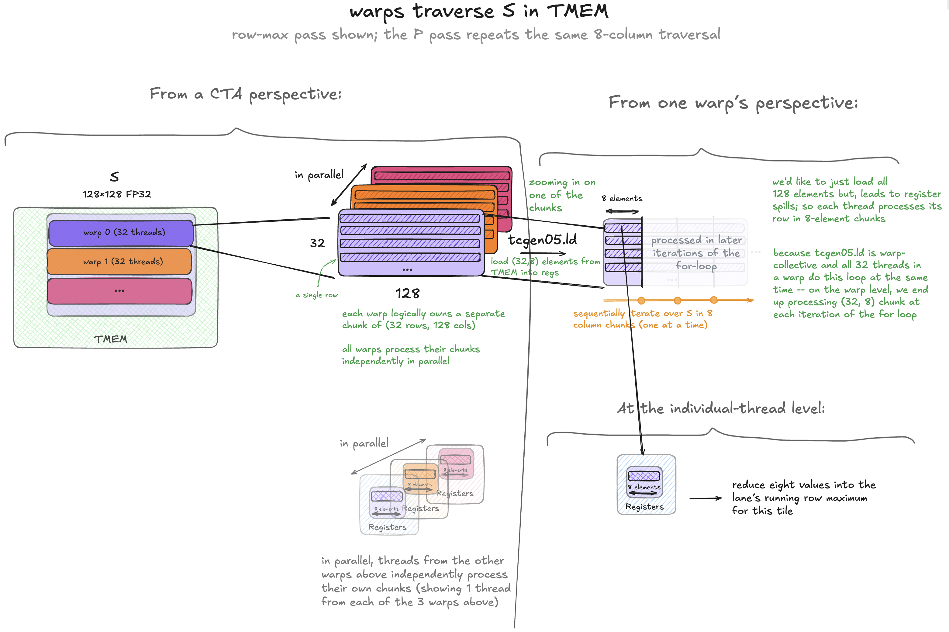
Only tcgen05. family of instructions can access TMEM, regular load/store instructions can’t.
So to compute the per-row max values, we first need to load values from TMEM (before computing their max),
so I’m using tcgen05.ld (stands for load) insturction to load values from TMEM into registers.
Let’s read this picture from left to right. We’ll follow the TMEM traversal at three levels: first the whole CTA, then one warp, and finally one thread within that warp. Our S tile in TMEM is (128 rows, 128 cols).
From the CTA perspective, the four warps split the 128 rows of S between them.
Each warp owns one 32, 128 row-chunk. That’s why our Kernel 1 has 4 warps
(to cover all 128 rows of S in 32-row chunks, so all 128 rows can be processed in parallel).
But each warp does not read it’s entire 32, 128 chunk at once.
This leads to register spills (not enough registers to hold all these four 32, 128 chunks in regs,
so compiler writes some of them to global memory which is incredebly slow).
To avoid this, each of the 4 warps iterates over its 32, 128 chunk in smaller steps, (32, 8) at a time.6
So there’s a for loop over TMEM columns.
Zooming into one warp: on each loop iteration, the warp loads a (32 rows, 8 cols) chunk from TMEM using tcgen05.ld.
All 32 threads participate in one load instruction (tcgen05.ld is “warp collective”).
This load distributes the chunk’s 32 rows we’re loading across the warp’s 32 threads, one row per thread.
So each thread in a warp receives the eight FP32 values from its row.
And tougether, the 32 threads in a warp hold the entire (32, 8) chunk.
From one thread’s perspective, at each iteration of the loop it keeps following the same row and receives 8 values at a time. And iterates over its 8 values, keeping the largest value it has seen so far.
In other words: The load is warp-collective, but the row computation is thread-local.
Each thread sees all 128 scores in that row, 8 at a time.
So each thread independently computes its row’s maximum in the first S pass.
That’s why each thread can keep its own tile_rowmax scalar in a register.
Each thread keeps working on the same query row throughout the K/V loop. Its rowmax and rowsum carry over between iterations, while tile_rowmax and tile_rowsum are recomputed for each tile.
Across all 4 warps, one iteration therefore processes a (128, 8) chunk of S.
Then the loop moves 8 columns to the right and repeats.
After 128/8=16 iterations, the 4 warps traversed all 128 columns of S.
At the end of the loop, each thread in a warp holds the max value for a given TMEM row.
In code, we call tcgen05::ld_32x32b_x8 helper:
.32x32b means load 32 TMEM rows with one 32-bit value per row;
.x8 repeats that shape across eight columns, all within a single tcgen05.ld instruction.
So each thread therefore gets eight 32-bit row values into eight of its registers.
That’s the (32,8) chunk shown in the diagram earlier.
Here is that first S pass in code. Each thread keeps its own tile_rowmax, updating it as it moves through the chunks.
float tile_rowmax = -FLT_MAX;

for (int score_n8 = 0; score_n8 < BLOCK_N / 8; ++score_n8) {
    // 8 FP32 temporaries per lane
    float s8[8];

    int addr = ... // covered below
    tcgen05::ld_32x32b_x8(addr, s8);

    for (int i = 0; i < 8; ++i) {
        tile_rowmax = fmaxf(tile_rowmax, s8[i]);
    }

}
Now, how do we tell that instruction which chunk to read?
Our S tile is [BLOCK_M, BLOCK_N] = [128,128], mapped to TMEM rows and columns respectively.
As shown earlier, the four warps cover separate 32-row regions, while each warp’s loop advances across columns.
A TMEM address is a 32-bit value containing two coordinates, rather than an ordinary byte address:
[ upper 16 bits: row ][ lower 16 bits: column ]
PTX calls a TMEM row a “lane.” For our load, these coordinates specify the starting row and column of the whole warp’s chunk. We don’t specify a separate row and column for each thread.
We construct that address like so:
// first row of this warp's region:
// 0, 32, 64, or 96, depending on the warp_id
int row_base = warp_id * 32;
// bitshift to the upper 16 bits
int trow = row_base << 16;

// inside the loop over S columns
int taddr =
    trow                // starting row, encoded in the upper bits
    + taddr_s           // starting column of S
    + score_n8 * 8;     // current chunk's column offset within S
The << 16 moves row_base into the upper 16 bits, leaving the lower half zero.
The column number already occupies the lower 16 bits because its numeric value is small, so its upper half is zero (needs no shifting).
To visualise it a bit (each bracket represents 16 bits):
row_base << 16:  [row_base][  0   ]
column:          [   0    ][column]
sum:             [row_base][column]

(here, column = taddr_s + score_n8 * 8)
Because the two fields don’t overlap, regular addition combines the row and column into one TMEM address.
Note, all 32 threads pass the same taddr. For this load shape, hardware
uses each thread’s lane ID to give it the values from row row_base + lane_id.
We do not add lane_id to the address ourselves (unlike ordinary per-thread addressing with ld.global).
For example, for row_base = 32:
- lane 0 receives values from row 32
- lane 1 receives values from row 33
- …
- lane 31 receives values from row 63
This is what’s meant by a warp-collective load: all 32 threads in a given warp participate in the same load instruction. Here, they all use the same taddr, but each receives eight values from its own row.
As the loop advances, trow stays fixed while the column offset increases by eight.
Before the second S pass: update the running rowmax
Now that we’ve computed this S tile’s per-row maxes, we need to update the running rowmax and rowsum, as per the online-softmax definition. The first S pass found tile_rowmax, the maximum for this row in the current S tile. But the second pass uses the running maximum, which also accounts for previous K/V tiles. Before the second pass, we combine tile_rowmax with the previous rowmax, and also rescale the old rowsum. These are per-thread scalar updates in registers, not another pass over S.
We take the larger of the two maxima and compute the rescale factor:
float new_rowmax = fmaxf(rowmax, tile_rowmax);
float rescale = __expf(rowmax - new_rowmax);

rowmax = new_rowmax;
rowsum *= rescale;
If the current tile raises the running rowmax, the old rowsum was computed using the previous maximum. So, we multiply it by rescale so those earlier contributions match the updated maximum.
The second S pass will use this updated rowmax to produce P. The same rescale factor must also be applied to old O, covered later in subsection ii.
Second S pass: produce P and update rowsum
Now that we have the updated running rowmaxes, let’s make the second pass over S. We reread S in chunks and subtract those rowmaxes from the scores, so we can safely exponentiate the results to produce unnormalized P.
We repeat the same TMEM traversal as in the first pass, so there’s no separate traversal diagram. What changes is what each thread does with its eight loaded values: subtract the updated running rowmax, exponentiate, add the results to the row’s sum, and write P into SMEM.
Let’s look more closely at how this second pass writes P into SMEM.
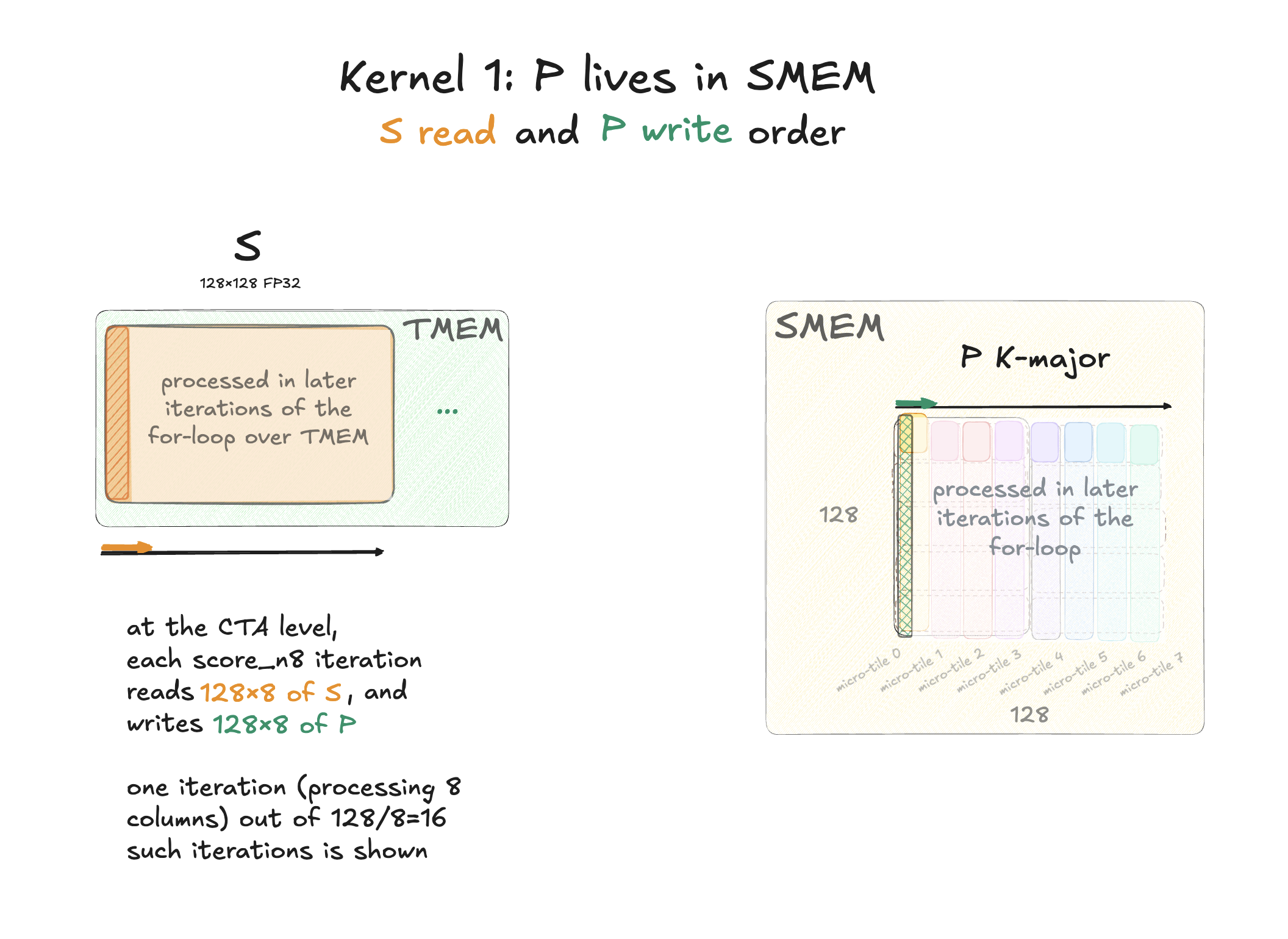
For each chunk of S we read, we produce a corresponding chunk of P and write it into the K-major SMEM layout. This is the layout the later P@V MMA expects.
Each iteration of the second S pass produces 8-column chunk of P. Two neighboring chunks make up one 16-column P micro-tile consumed by the later PV MMA micro-step.
S itself stays unchanged in TMEM. We store P in the same SMEM buffer that previously held K. K is already dead after QK, so it is safe to reuse that storage for P.
Here is the second S pass in code, reading S from TMEM and writing P into SMEM.
int row = row_base + lane_id;
float tile_rowsum = 0.0f;

for (int score_n8 = 0; score_n8 < BLOCK_N / 8; ++score_n8) {
    float s8[8];

    int addr = ...; // same TMEM address calculation as the first pass
    tcgen05::ld_32x32b_x8(addr, s8);

    for (int i = 0; i < 8; ++i) {
        float p = __expf(s8[i] - rowmax);
        tile_rowsum += p;

        // write P into K-major SMEM
        int col = score_n8 * 8 + i;
        int p_idx = idx_kmajor_w8(BLOCK_M, row, col);
        P_smem_ptr[p_idx] = __float2bfloat16_rn(p);
    }
}

rowsum += tile_rowsum;
writing P into SMEM
idx_kmajor_w8 computes where each P value belongs in our familiar K-major SMEM layout (which we already covered in Section A), needed for the later PV matmul.
The helper implementation itself isn’t too important to understand, ignore it.
We need row variable here becuase unlike the warp-collective TMEM load, these are regular per-thread SMEM stores.
ii) Rescaling O
Now let’s return to the O-rescale pass, which happens between the two S passes in the kernel code.
Earlier we computed the new max basis. But the old O tile is still in the old basis. So before we do O += P @ V we need to rescale O.
In the online-softmax algorithm, PV is generally unsafe to accumulate into O, until old O is in the current max basis.
Earlier we updated the running rowmaxes to include the current S tile. Changing the rowmax changes the scale of the unnormalized P values, so it also affects the P@V contributions accumulated in O. We rescale the old O so those earlier contributions match the updated rowmax before adding the current P@V contribution.
This is standard online-softmax formulation, the only changes here is that I’m mapping it to the Blackwell B200 hardware.
As mentioned earlier, the rowsum and rowmax are per-thread scalars. O is different, it’s a full [BLOCK_M, HEAD_DIM] partial accumulator tile stored in TMEM.
So, to rescale these values: we need to read columns of TMEM holding O,
then rescale them (by the rescale factor we just computed from the old and new rowmaxes),
then write the rescaled values back to TMEM.
We need to write O back because this is still a running partial O, not the final output.
So that later PV matmul can accumulate its partial into the udpated basis.
Each thread uses its own rescale factor for all the values in its O row. We skip this pass on the first K/V iteration, because there is no previous O yet. The first PV microstep initializes O.
float o8[8];

for (int out_n8 = 0; out_n8 < HEAD_DIM / 8; ++out_n8) {

    // same TMEM address calculation as before, now for O
    int taddr =
        trow                // starting row, encoded in the upper bits
        + taddr_o           // starting column of O
        + out_n8 * 8;       // current chunk's column offset within O
    tcgen05::ld_32x32b_x8(taddr, o8);

    for (int i = 0; i < 8; ++i) {
        o8[i] *= rescale;
    }

    tcgen05::st_32x32b_x8(taddr, o8);
}
This uses the same 4 warps, row ownership, and 8-column chunks as the S traversal covered above.
The new part is that after rescaling the values in registers, we use
tcgen05.st to write the corrected O back into TMEM.
The store-completion wait and synchronization are omitted here, the full kernel completes the O stores before PV uses the accumulator.
With P ready in SMEM and O rescaled in TMEM, Section C can now add P @ V into O.
C) P@V (explaining MN-major)
Inside one K/V-loop iteration — Step 3 of 3.
Above we covered how P tile is produced, now we need to matmul it with V tile. Turns out, unlike for the Q, K, and P (which all use the same K-major SMEM layout, as dicussed above), V uses a different SMEM layout. So that’s our next topic of discussion.
For our Kernel 1, P_tile is produced into SMEM by softmax, so it is not shown in the global-memory view below.
In the kernel, V is loaded alongside K before QK. I explain V’s copy here so we can discuss its SMEM layout together with the PV matmul that uses it.
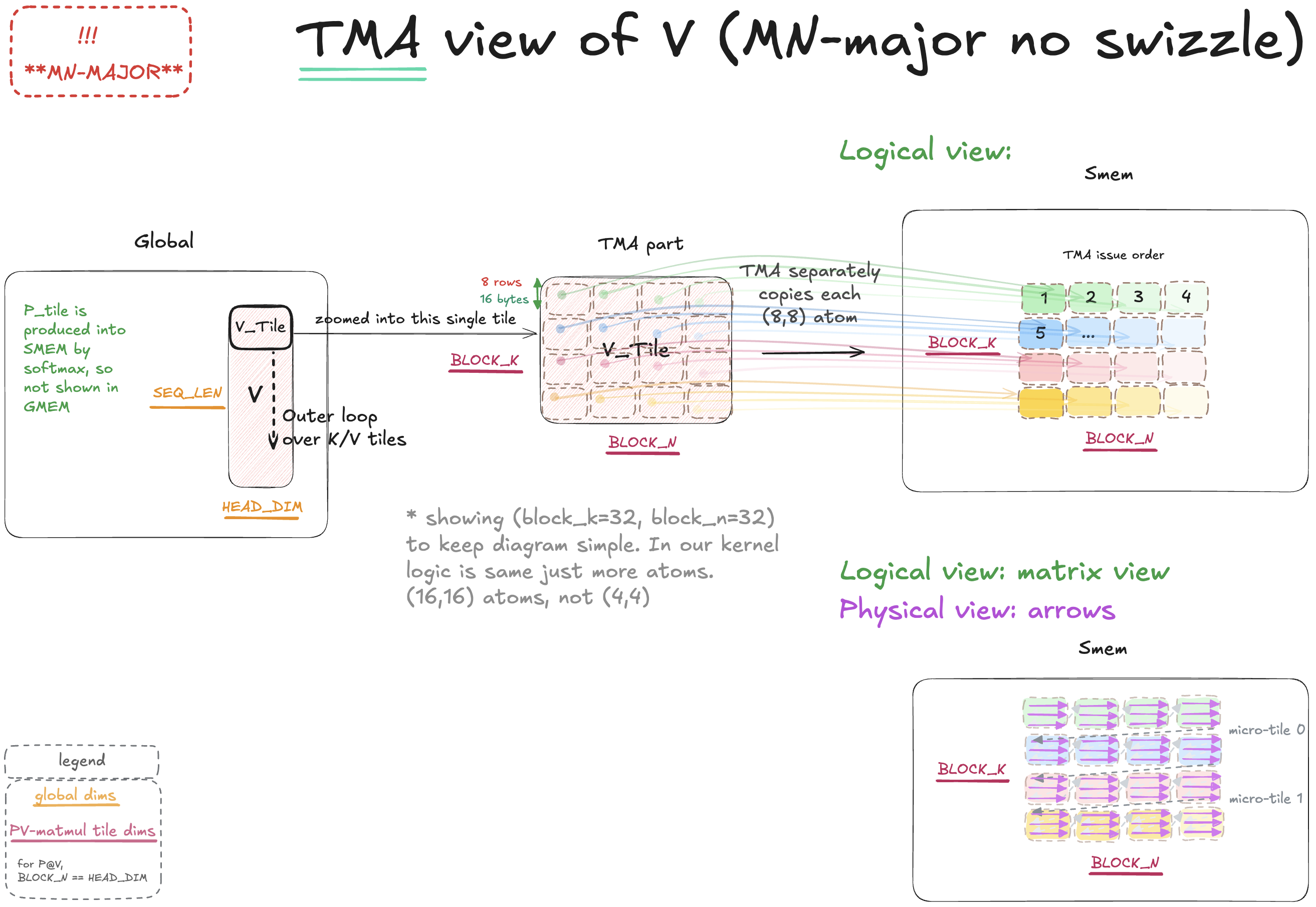
Note: The matmul diagrams and code snippets use matmul-centric dimension names. Actual kernel source keeps fixed attention-tile names.
For the PV matmul diagrams below, I name dims using conventional matmul dim names: P[M,K] @ V[K,N] = O[M,N]
Let me step back for a moment and explain why I name axes M, N, and K. I use conventional M/N/K names separately for each matmul, because for each matmul standalone, it makes its input shapes easier to read. So these M/N/K are a matmul-centric naming choice, not inherent properties of global tensors (Q, K, P, or V).
That is why the same source dimension can have different local names in QK and PV. So, K-dim means the reduction dim of the current matmul: features for QK, but the K/V tile rows for PV. Now back to our larger, PV matmul discussion.
Q, K, and V start in the same global-memory layout, but in the kernel, we lay them out differently in SMEM depending on how each MMA will consume them. Why do I use k-major layout for Q tile, K tile, and P tile, but use a different layout (discussed below) for the V tile?
Becuase QK needs K viewed transposed, while for PV the inner dimensions already match, so V does not need a transpose. More concretely:
QK: Q[M,K] @ K[N,K].T
PV: P[M,K] @ V[K,N]
For QK, K is stored as [N,K], MMA consumes its B operand as logical [K,N].
So I use K-major for K. This lets MMA interpret the stored K tile as the logical
transposed operand, without first constructing a separate transposed K tile.
For PV, V is already in the [K,N] orientation needed by the MMA B operand, so I use MN-major for it.
This lets MMA consume V directly, without first transposing V tile.
P is the [M,K] A operand, so it remains K-major.
In other words, for the stored tile views used in these diagrams, my shortcut is:
- K-major: reduction K is on the right, as in Q[M,K], K[N,K], or P[M,K].
- MN-major B: reduction K is on the left, as in V[K,N].
It’s only a shortcut I use for reading these operand views, not formal definition of K-major and MN-major layouts.
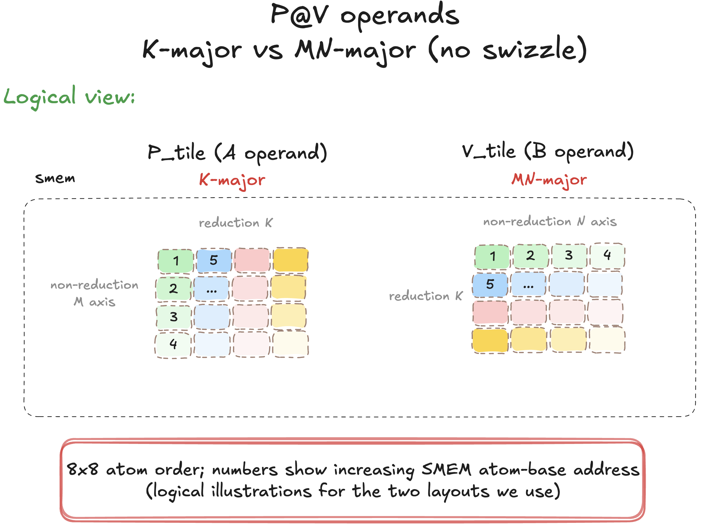
These are the two operands of the same PV MMA. tcgen05.mma lets us choose the major mode of A and B independently, so P can be K-major and V can be MN-major.
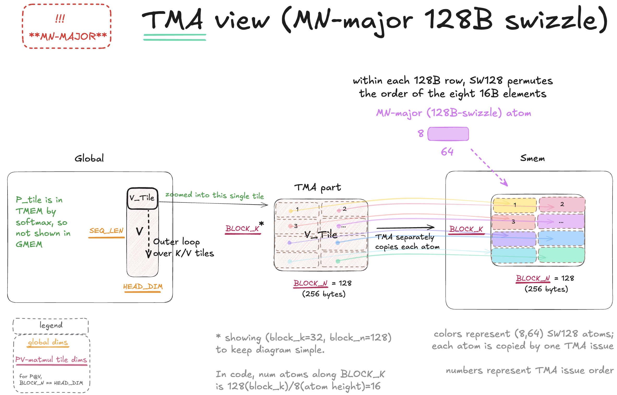
P on the left uses the same K-major atom order as Q in Section A. The numbers show increasing SMEM addresses. Both layouts use (8,8) atoms. What changes is which atoms are stored back-to-back, and that determines how much data we copy per TMA call.
Remember that for Q, one TMA call copied a whole vertical slice and placed its atoms in the correct order. V uses a different SMEM layout, with a different atom order, so we need to rethink how much data each TMA call should copy.
Why not copy V in larger slices, as we did for Q?
For Q, the atoms of one vertical slice are stored back-to-back in SMEM. So one TMA call can copy that whole slice.
For V, look at the atom order in the diagram: we place atoms across the first eight-row stripe, then move down to the next stripe. So the atoms of one vertical slice are separated by other atoms in SMEM. So copying the whole vertical slice in one TMA call would put its atoms in the wrong places in SMEM.
But why not copy a whole horizontal stripe instead? Our simple, unswizzled 2D TMA copy would store that rectangle row by row. We would get a simple row-major in SMEM (one full row of values, then the next full row). But our layout needs all eight rows of one (8,8) atom before the next atom.
So we copy one atom at a time and explicitly choose where each atom lands in SMEM.
Here is the V-copy loop, slightly simplified. Unlike the Q copy, each TMA call copies one (8,8) BF16 atom, rather than a full-height vertical slice.
V_tmap contains the same kind of metadata as Q_tmap used earlier (global-memory address, dtype, dims, strides), but its copy shape is now (8 rows, 8 columns). kv_row0 is the current V tile’s first global row. Using the diagram’s names, this V tile is (BLOCK_K rows, BLOCK_N columns).
int ATOM_BYTES = (8 * 8) * 2;          // one 8x8 BF16 atom
int STRIPE_BYTES = (8 * BLOCK_N) * 2;  // one full 8-row stripe

// one thread issues all these TMA copies;
// barrier setup and completion wait omitted

// move down V, 8 rows at a time
for (int row8 = 0; row8 < BLOCK_K / 8; ++row8) {

    // copy one (8,8) atom per iteration, moving from left to right
    for (int col8 = 0; col8 < BLOCK_N / 8; ++col8) {

        // starting row and column of this (8,8) atom in global V;
        // element coordinates, not byte offsets
        int src_row = kv_row0 + row8 * 8;
        int src_col = col8 * 8;

        // V_smem is the starting byte address in SMEM
        int dst_smem = V_smem
                     + row8 * STRIPE_BYTES
                     + col8 * ATOM_BYTES;

        tma::copy_2d_gmem_to_smem(
            dst_smem, &V_tmap, src_col, src_row, mbar_addr);
    }
}
The inner loop places complete atoms next to each other in SMEM. Then the outer loop moves down to the next 8-row stripe, and we repeat. These offsets construct the MN-major physical layout shown above.
For our (128,128) V tile, the loops issue (16 copies down, 16 copies across) = 256 copies. We don’t loop over the individual elements, each call copies all 64 values of its (8,8) atom.
We now know how both PV operands are prepared in SMEM: P by softmax (our previous section B), and we’ve just discussed how to separately copy V into SMEM. Let’s see how MMA consumes them.
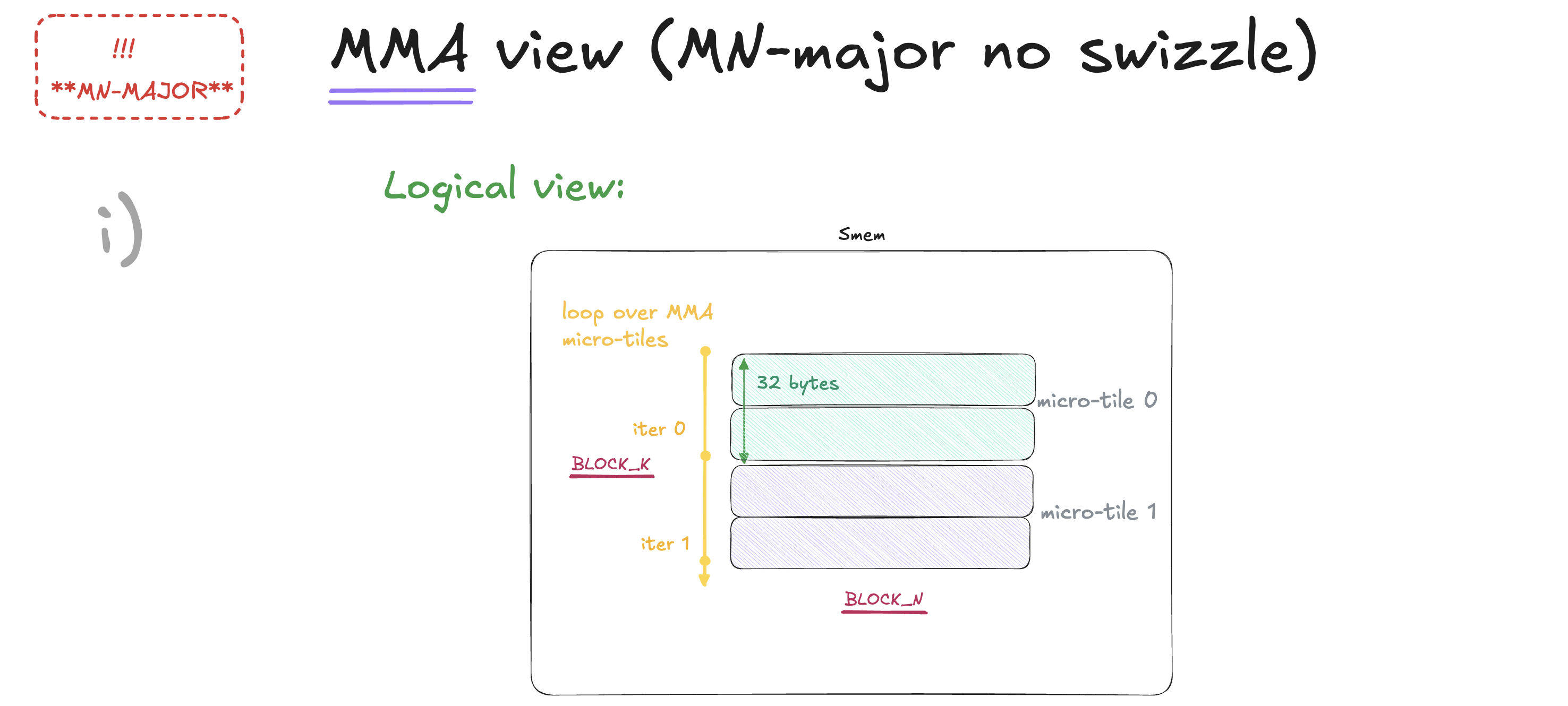
Same basic idea as for QK (explained in earlier section A):
our reduction dim labeled BLOCK_K in this diagram
has 128 BF16 elements, but one tcgen05.mma issue consumes only MMA_K=16 BF16 elements.
So PV is split into 128 / 16 = 8 MMA microsteps.
For simplicity, I only show 2 of these microsteps.
In this V view, reduction K is vertical. So one microstep consumes two neighboring 8-row slices.
Along BLOCK_K, each microstep consumes 16 BF16 elements. Since each BF16 element is 2 bytes, that is the 32 bytes shown in the diagram.
The PV loop follows the same structure as QK. P uses a K-major descriptor, but what’s different is that V uses an MN-major descriptor. Instruction descriptor i_desc_pv specifies the MMA shape, dtypes, and those operand modes.
Each PV microstep consumes 16 columns of P and the matching 16 rows of V, contributing to the same O tile.
// P uses SMEM storage previously used by K
int P_smem = K_smem;

uint64_t p_desc = noswizzle::desc_kmajor(P_smem, BLOCK_M);
uint64_t v_desc = noswizzle::desc_mnmajor(V_smem, BLOCK_N);

// MMA_K = 16 BF16 values; MMA_K_BYTES = 32.
// descriptor addresses are encoded in 16-byte units
uint64_t p_desc_step = (BLOCK_M * MMA_K_BYTES) / 16;
uint64_t v_desc_step = (BLOCK_N * MMA_K_BYTES) / 16;

// one thread issues all MMA micro-steps
for (int k = 0; k < BLOCK_K / MMA_K; ++k) {

    // initialize O only on very first PV microstep,
    // every later microstep accumulates into existing O.
    // (kv_tile is zero-based index of the current K/V tile).
    int enable_input_d = (kv_tile == 0 && k == 0) ? 0 : 1;

    tcgen05::mma_f16(
        taddr_o, p_desc, v_desc, i_desc_pv, enable_input_d);

    p_desc += p_desc_step;  // next 16 columns of P
    v_desc += v_desc_step;  // next 16 rows of V
}

// track completion of all 128/16=8 PV microsteps
tcgen05::commit_arrive(mbar_addr);
One difference from QK is initialization condition. QK starts a fresh S tile on every K/V iteration. But O must keep contributions from previous K/V tiles (already rescaled in Section B). So, only the first microstep of the first K/V iteration initializes O, all later microsteps accumulate into it. On that first K/V iteration, the kernel also skips O rescaling (there is no previous O to rescale yet).
The loop advances both descriptors to the next pair of micro-tiles. Now let’s zoom into the V descriptor: where does its base point, and how does MMA locate the other atoms in that micro-tile?
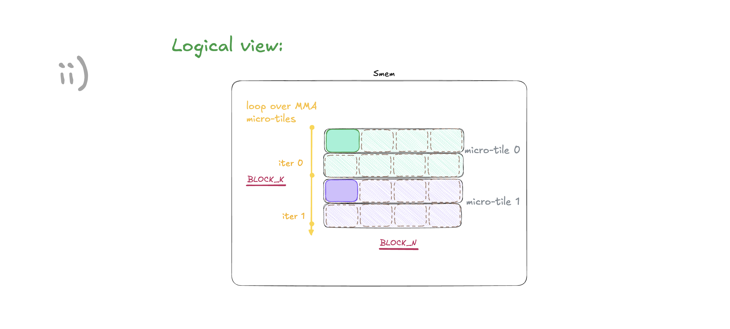
For each PV microstep, the V operand descriptor base points at the first (8,8) V atom
in that 16-row chunk.
For microstep 0, the V descriptor base is the green highlighted atom. Our loop over micro-tiles then advances descriptor to the next 16-row chunk. For microstep 1, the V descriptor base becomes the purple highlighted atom.
The next figure shows how LBO and SBO cover the remaining atoms in the same micro-tile from that descriptor base.
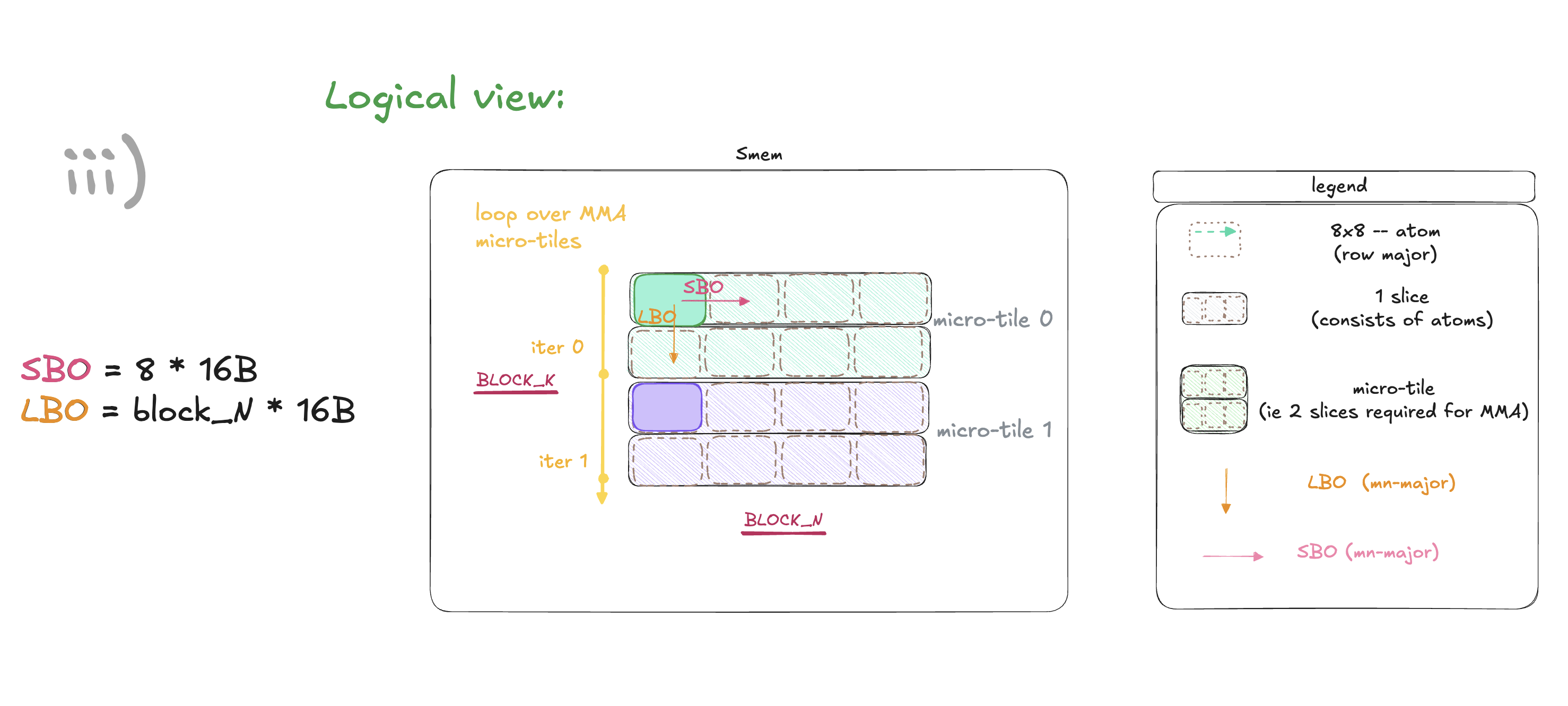
For each PV microstep, descriptor base points at the first atom in the first 8 row V slice.
LBO reaches the corresponding atom in the second 8 row slice, while SBO steps across the 8 column wide atoms along N.
These are the same offsets we used in the V-copy loop. For our 128-column V tile:
SBO = ATOM_BYTES   = 8 * 8 * 2       = 128 bytes
LBO = STRIPE_BYTES = 8 * BLOCK_N * 2 = 2048 bytes
So the copying loop and the MMA descriptor agree on where the atoms live: TMA places them at these offsets, and MMA uses those same offsets to find them.
Using that starting address, the two offsets, and the MMA shape, one
tcgen05.mma issue covers complete 16row V micro-tile.
Then the loop advances P’s descriptor to the next 16 columns and V’s descriptor to the matching next 16 rows.
For V, the next micro-tile starts 16 rows lower – two 8-row stripes down. So we advance its base address by 2 * STRIPE_BYTES = 4096 bytes.
Descriptor addresses are encoded in 16-byte units, so dividing by 16 gives the encoded v_desc_step used in the code above.
Zooming back out: one K/V iteration
In Chapter 1’s Sections A, B, and C, we zoomed in the individual steps inside one K/V-loop iteration. Now let’s zoom back on the level of a complete KV-loop iteration.
One thing the diagrams above omit is synchronization.
TMA loads and tcgen05.mma are asynchronous.
But in Kernel 1, we immediately wait on every major handoff:
load the current K/V tile and wait,
run QK and wait,
do the row work,
then run PV and wait.
Only after PV finishes we start loading the next K/V tile.
So this baseline still runs one semantic stage after another. Only one K/V tile is live, and there is no useful overlap between the K/V load, QK, row work, and PV yet. Later kernels start overlapping these stages.
In the source, mbarriers tell us when the asynchronous TMA and MMA work has completed.
__syncthreads() only waits until all CTA threads reach that point;
it does not wait for the asynchronous TMA or MMA work to finish.
Epilogue: after we finish entire K/V loop, we read O from TMEM using the same four warps, eight columns at a time. Each thread divides the values from its row by its final rowsum, converts them to BF16, and writes them to global memory. Unlike the earlier O-rescale pass, here we’re writing the final output to global memory (not back into TMEM).
KERNEL CHECKPOINT
This blog is not diagrams only, the code is equally important.
See 1_baseline.cu
It follows the same exact sequence as we studied:
- each CTA holds a single Q tile; loops over all K, V tiles
- S=Q@K.T (tcgen05 in microtiles, K-major layout)
- S->P (accessing TMEM)
- O+=P@V (tcgen05 in microtiles, MN-major layout)
Now, familiarize yourself with the code.
Performance so far
This table will grow by one row after every chapter. Stock FA4 (cute DSL) is 100%. Each value is the median of six same-run ratios; every benchmark invocation measured this kernel and stock FA4 on the same B200.
| Kernel | Change | 4k | 8k | 16k |
|---|---|---|---|---|
| 1 | Baseline | 14.2% | 14.1% | 13.7% |
⭐ Star the repo so you have all the kernels at hand as we go through the later chapters.
More ML systems articles, videos, and code are coming: LinkedIn · X · YouTube
Chapter 2 – move P from SMEM to TMEM
In kernel 1, the second softmax pass reads S from TMEM, converts it into the unnormalized probabilities P, and writes P into the SMEM buffer that previously held K (K buffer is dead after QK, so we safely re-used it for P).
Kernel 2 changes where P lives. Instead of writing P fragments to SMEM, we write them back into the TMEM. That’s the main change introduced by kernel 2.
This change doesn’t reduce SMEM usage, but it prepares for later optimizations. By storing P into K’s dead SMEM slot Kernel 1 coupled their lifetimes: K is no longer needed after QK, but its slot remains used by P until PV consumes it, which is suboptimal. We could give P a separate SMEM buffer, but we’ll need almost entire SM’s SMEM budget for our future optimizations. Instead, kernel moves P to TMEM, separating their lifetimes without allocating more SMEM. In later chapters, this lets us use that decoupled P and K lifetime for additional optimizations.
The allocated SMEM does not reduce, kernel still needs Q,K,V storage.
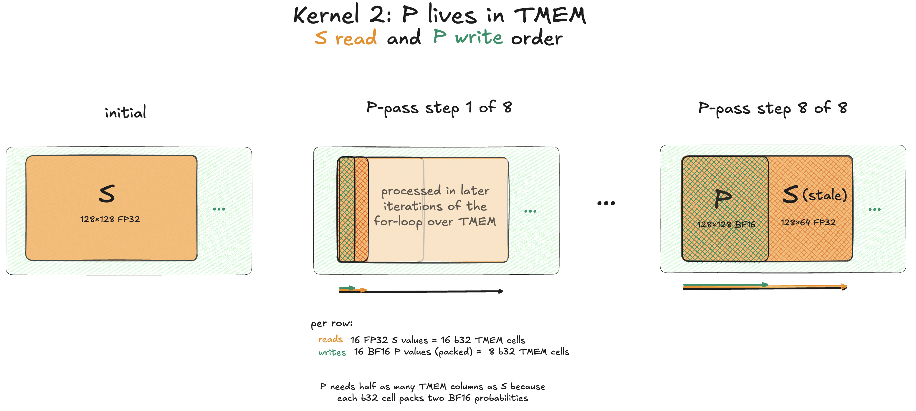
As an optimization we write P directly into the allocation that held S so P needs no additional TMEM allocation. (because we can safely overwrite the elements of S which the second pass over TMEM already consumed).
So, in kernel 2, the same TMEM slot changes meaning over time:
- after QK: the slot holds FP32 S
- softmax pass 2: consumed S chunks are overwritten by packed BF16 P
- PV: the slot is consumed as P
This does create the coupling of S and P lifetimes, but as you will see later is not as problematic as the coupling of P and K lifetimes.7
TMEM is organized as 32-bit memory cells yet our P values are bf16, so 2 of our P values can be packed into one TMEM cell. Likewise, S contains FP32 values, so one score (one value in the S matrix) occupies one b32 TMEM cell. So, P uses half of TMEM columns as S.
The figure shows one logical 16-score step, shown as differently colored arrows.
In code, that step is implemented using two tcgen05.ld.x8 loads (shown as orange arrows),
followed by one tcgen05.st.x8 store (shown as green arrows).
Kernel 1 processes P in width-8 chunks. Kernel 2 groups two of these chunks into one iteration,
per row, loading 16 FP32 S values and producing 16 BF16 P values.
The width-16 grouping is not fundamental.8
Remember from kernel 1, when producing P we iterate over TMEM in chunks (see the relevant diagram from the previous chapter), this is very similar to chapter 1. What’s new in ch-2, is we store the resulting P chunk in TMEM (by packing 16 P values into 8 b32 TMEM cells). So S-read pointer advances by 16 columns, while the packed-P-write pointer advances by only eight. Thus, each P write remains behind the read pointer and overwrites only scores already consumed by this second TMEM pass. So when producing P and writing it into TMEM (in chunks) we are not at the risk of clobbering unread S values, as also shown on the diagram.9
Our S takes up 128 TMEM columns, and as mentioned we read in 16-column chunks, so we need 128/16=8 iterations to cover all TMEM S columns. After all eight steps, the lower 64 b32 columns contain complete 128-column BF16 P tile. So P doesn’t overwrite the entire S buffer, but only half of it. The remaining half contains stale S values that are never read again. The next QK (in the next iteration of the KV for-loop) fully overwrites the entire S/P slot with S(i+1).
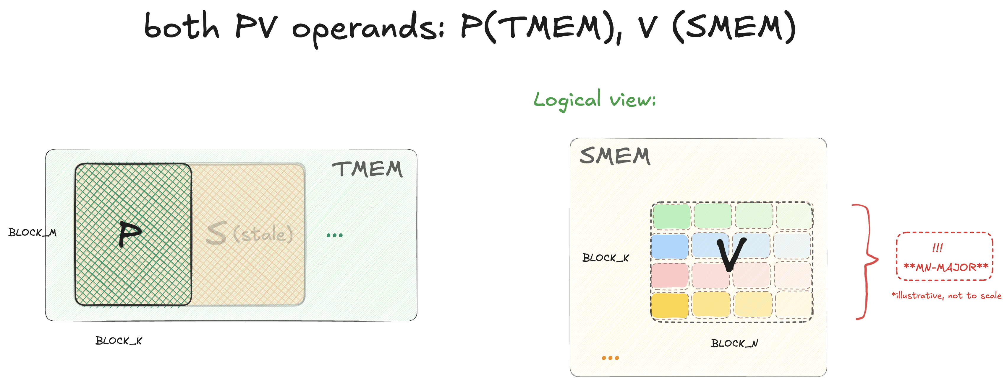
PV matmul doesn’t change:
P[BLOCK_M, BLOCK_K] @ V[BLOCK_K, BLOCK_N] -> O[BLOCK_M, BLOCK_N]
Only the source of P (the A operand) changes. In kernel 1 both P and V were consumed from SMEM. In kernel 2, P is consumed from TMEM, V from SMEM.
In kernel 1, P needed a K-major SMEM layout and SMEM descriptor. In kernel 2, P is identified directly by a TMEM address, and we no longer use the SMEM descriptor for P.
K-major and MN-major are SMEM-only-layouts and are not used for TMEM operands. V remains the MN-major SMEM B operand.
At this point we’ve discussed how P is produced and written to TMEM (as oppose to written in SMEM, as in Chapter 1). Let’s now discuss the P@V matmul again, but now one of the operands (P) will come from TMEM.
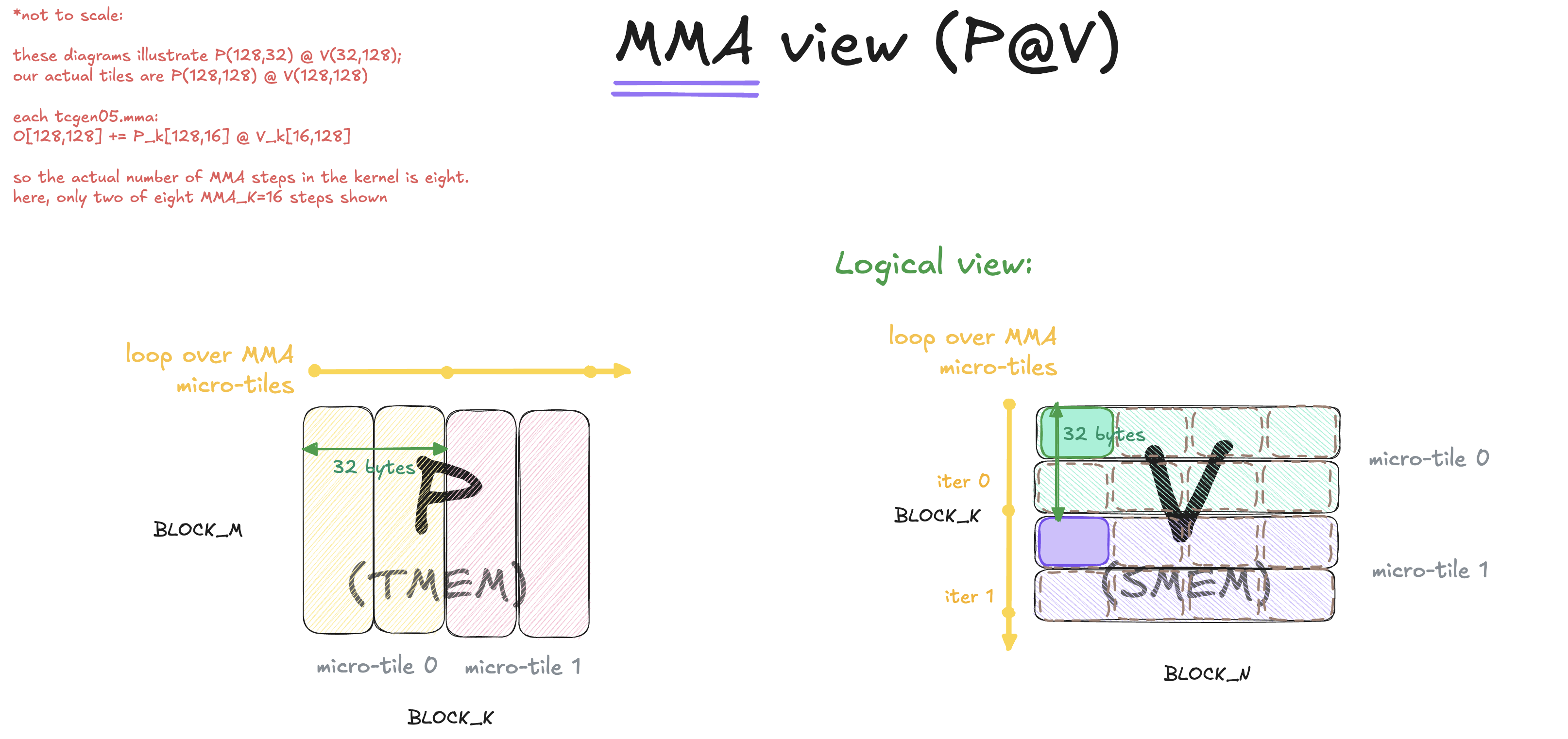
Keep in mind all my MMA-related dims in the diagrams use conventional local matmul notation: A[M,K] @ B[K,N] = C[M,N]
So, PV reduces over BLOCK_K = 128.
Same as in chapter 1, each MMA issue consumes matching MMA_K=16 micro-tiles of P and V:
P[:, 16k : 16(k+1)] @ V[16k : 16(k+1), :].
Eight MMA_K=16 issues cover the complete BLOCK_K=128 reduction.
To avoid clutter, the figure shows only the first two.
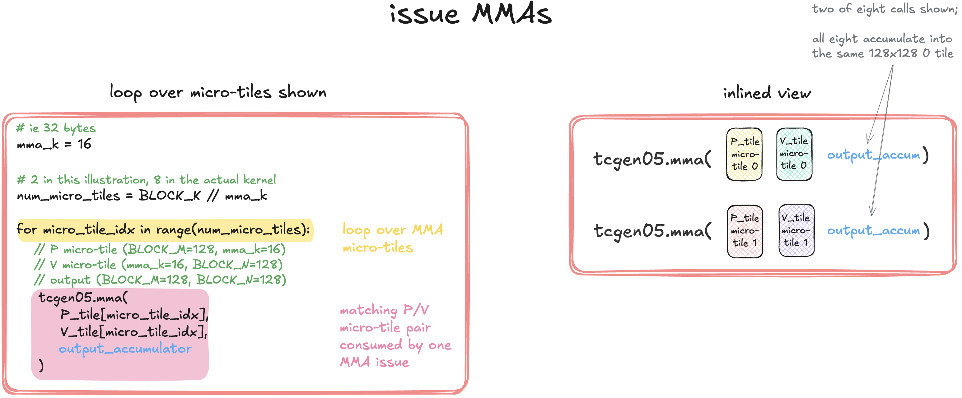
The loop follows the same logical MMA_K=16 micro-tile order as kernel 1, but selects P through TMEM addresses instead of advancing an
SMEM descriptor. taddr_p + k * 8 points to the base of the next 128x16 P micro-tile.
Within each row, its 16 BF16 values take eight b32 TMEM columns.
The V descriptor advances to the matching 16 rows, and every issue accumulates into the same O tile.
Because P is now produced with tcgen05.st, the row threads must wait
for those TMEM stores and fence before PV begins.
This is just a minor change to the publication mechanism.
So kernel 2 leaves the softmax math, PV reduction order, and high level schedule unchanged. Its only semantic change is: QK produces S in TMEM, softmax turns that storage into P, PV consumes P directly from TMEM.
KERNEL CHECKPOINT
See 2_p_to_tmem.cu and diff it against Kernel 1.
It follows the same exact sequence as we studied:
- softmax overwrites consumed S with packed BF16 P
- PV reads P from TMEM and V from MN-major SMEM
- P doesn’t reuse K’s SMEM slot
- the math and schedule unchanged
Now, familiarize yourself with the code.
Performance so far
| Kernel | Change | 4k | 8k | 16k |
|---|---|---|---|---|
| 1 | Baseline | 14.2% | 14.1% | 13.7% |
| 2 | P in TMEM | 15.1% | 15.0% | 15.0% |
This didn’t lead to a performance improvement, but these changes did uncouple K and P lifetimes, which will enable our later major optimizations.
I kept this as a separate step instead of folding it into Kernel 1 because writing P to TMEM introduces additional addressing, packing, and synchronization details. Kernel 1 already introduces enough new concepts, so I didn’t want to complicate it unnecessarily, and tried to keep the initial baseline simpler.
Chapter 3 – Swizzling
We already chose Q/K as K-major and V as MN-major based on how each source tile is consumed by its MMA (we covered this in chapter 1, revisit if you need a refresher). Kernel 3 keeps the same schedule and major modes, and only changes the swizzle mode (of each of the tiles independently): Q/K/V moves from no-swizzle to SW128 in SMEM, to reduce SMEM bank conflicts. P stays in TMEM, so swizzling is not applied to it.
There’s my resources explaining the motivation behind swizzling, I will not repeat it here, because our goals is understanding B200 related concepts, suffice to say swizzling permutes SMEM addresses within each atom so tensor core accesses map better across SMEM banks and avoid bank conflicts. I cover B200 specific details below (but not the generic swizzling expaliner).
Major mode and swizzling are two separate things (dicussed in chapter 1, revisit if you need a refressher). Major mode says which matmul dim is packed inside the 16B elements: K for K-major, or M/N for MN-major. Swizzling adds address permutation inside fixed-size atoms of that layout. So we first choose the major mode based on the operand’s role in the matmul. Once we also decided to use swizzling (SW128), the required atom shapes follow from the tcgen05 layout table below.
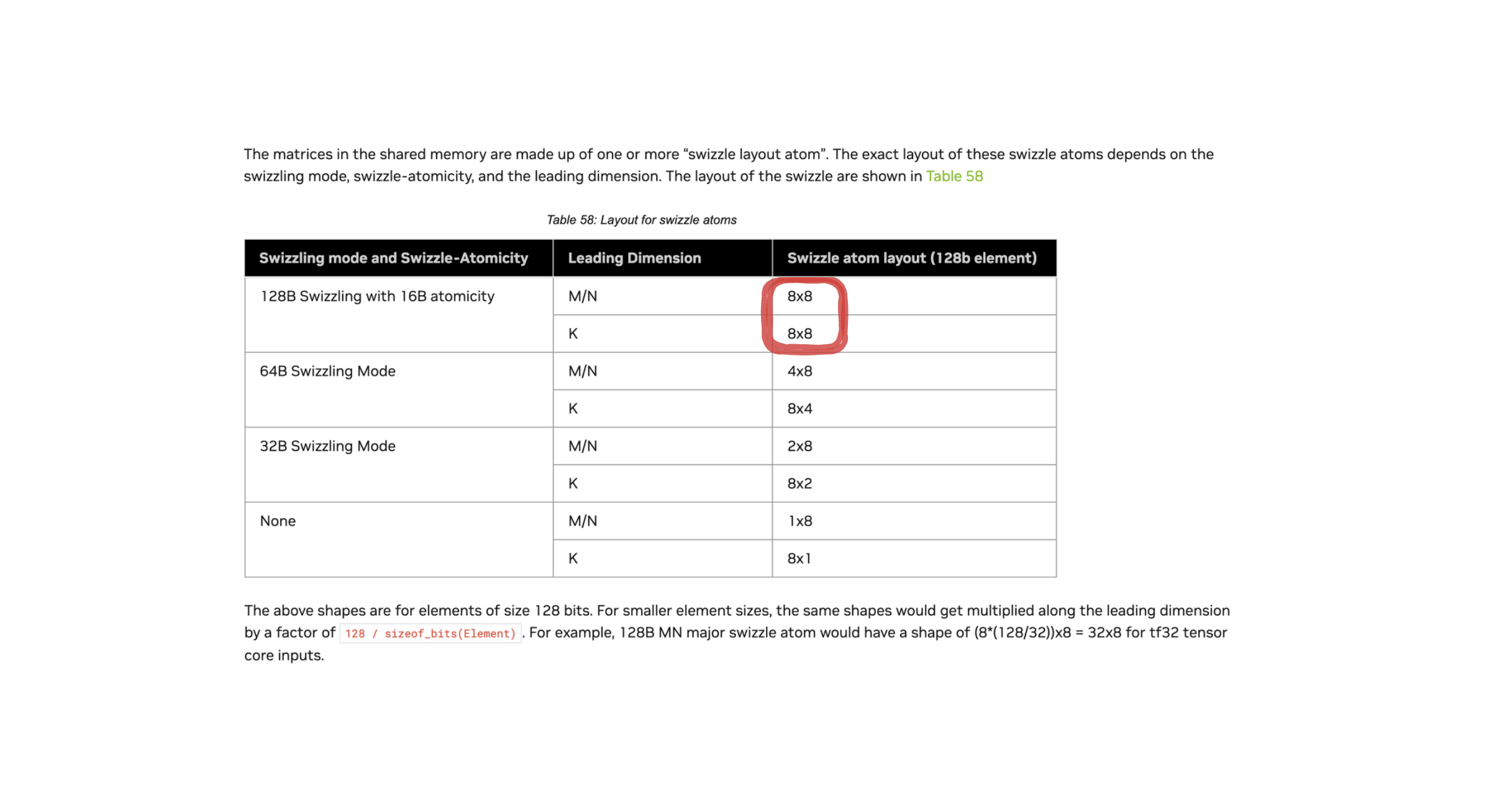
Let’s translate that table into BF16 elements, which is the dtype of our input tensors.
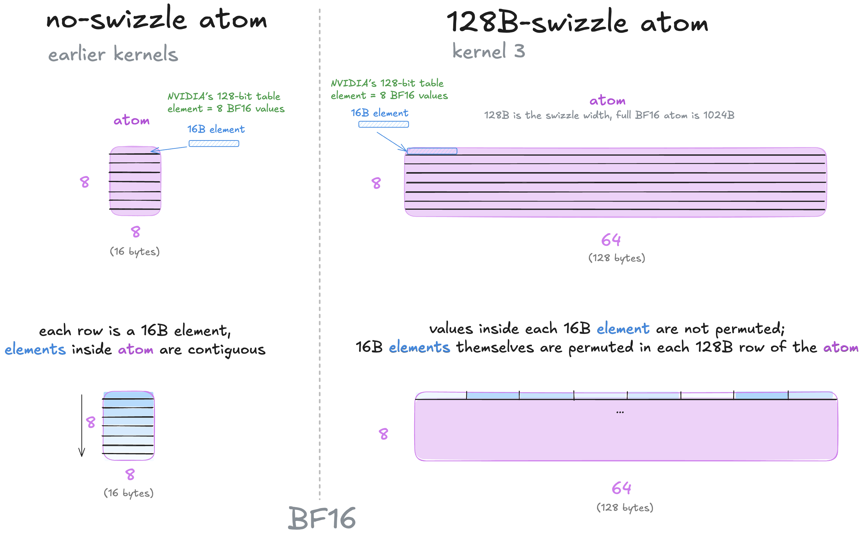
When we added swizzling, two points worth covering: (i) atoms got wider, and (ii) became swizzled inside. These two points are adresed below in order.
(i) atoms get wider
NVIDIA describes the tcgen05 shared-memory layout table in terms of 128-bit elements (16 bytes).
, not BF16 values.
One BF16 value is 16 bits, so one 128-bit element contains 128/16 = 8 BF16 values.
The docs say to expand only the leading dim in the atoms.
In the table, atom dims are ordered as (M/N, K), though this wasn’t immediately obvious 10.
So for K-major, K is the leading dim, which is 2nd axis:
(8,8) -> (8, 8*8) = (8,64) BF16
For Q/K, we already draw source tiles in [M/N,K] coordinates,
so their K-major atoms appear as (8,64).
For MN-major, M/N is the leading dim, which is the 1st axis:
(8,8) -> (8*8, 8) = (64,8) BF16
For V, the MN-major atom is (64,8) in NVIDIA’s [N,K] coordinates.
In the source V[K,N] logical views I draw, those axes are swapped, making it (8,64).
That’s why both atom types look (8,64) in my source-coordinate diagrams,
even though they are not the same layout.
For now, let’s first zoom into the K-major layout (used Q@K). We’ll later return to the MN-major layout (used for V in P@V).
(ii) swizzled inside
As far as I understand, with swizzling added, elements inside a 16B element are not permuted, 16B elements themselves are permuted.
We don’t care about exact row-by-row permutation, because we do not compute it manually. Instead, on blackwell we rely on a) TMA writes in swizzle-128B layout, and b) tcgen05 reads expecting swizzle-128B layout.
SMEM layout and the downstream MMA have to agree on layout, as we know from Chapter 1.
Concretely, we set CU_TENSOR_MAP_SWIZZLE_128B in TMA tensor maps, so TMA writes Q/K/V swizzled.
And then set the matching SW128 mode in the tcgen05 operand descriptors, so tcgen05 knows to consume the swizzled layout.
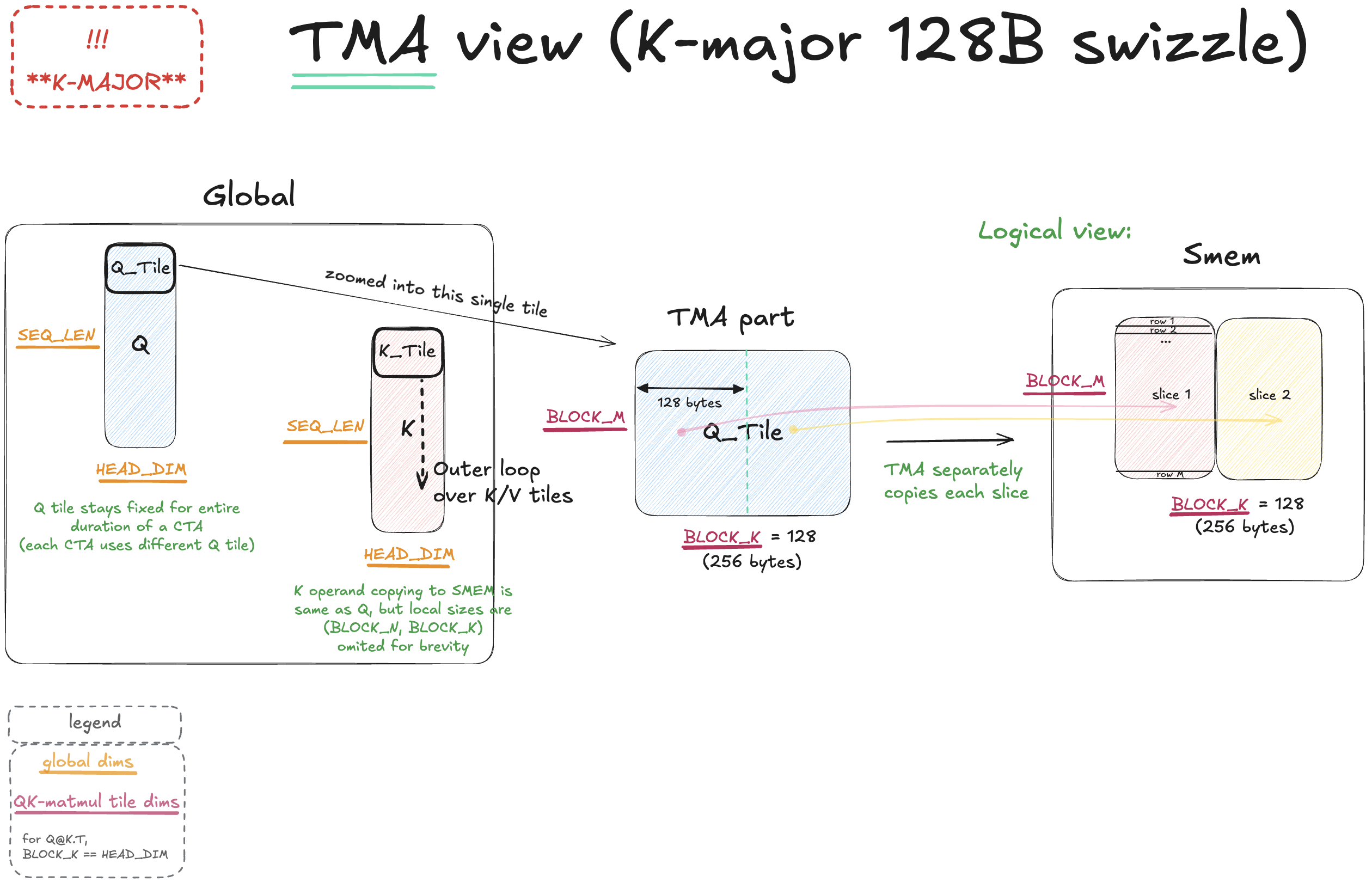
Let’s zoom into K-major layout first (used for both operands of Q@K.T).
When copying into SMEM we want to lay out our data according to (8,64) atoms as explained above.
One K-major SW128 atom is 64 BF16 elements wide (ie 128B).
But our full Q/K tile is HEAD_DIM=128 elements wide (ie 256B).
With a simple 2D SW128 TMA map that we use, we can’t copy the full 128-wide tile at once and ask TMA to treat it as two separately swizzled 128B regions. CUDA requires the inner dim of one SW128 TMA box to be at most 128B. In our Q/K tensor maps, that inner dim corresponds to HEAD_DIM (the horizontal dim in the figure). So we split HEAD_DIM into two 64-wide slices.
But it doesn’t mean we need one TMA issue per (8,64) atom.
The 128B restriction is only on the inner width.
Once the width is 64, the same TMA box can extend down all rows of the tile:
- Q copy:
(BLOCK_M, 64) - K copy:
(BLOCK_N, 64)
In this kernel, both tile heights are 128.
So one TMA issue copies one (128,64) slice,
containing 16 vertically stacked (8,64) atoms.
Above we discussed how we tell TMA to use swizzling when copying our data to K-major swizzled SMEM layout. But there’s the second part, which is: telling MMA how to consume the K-major siwzzled layout.
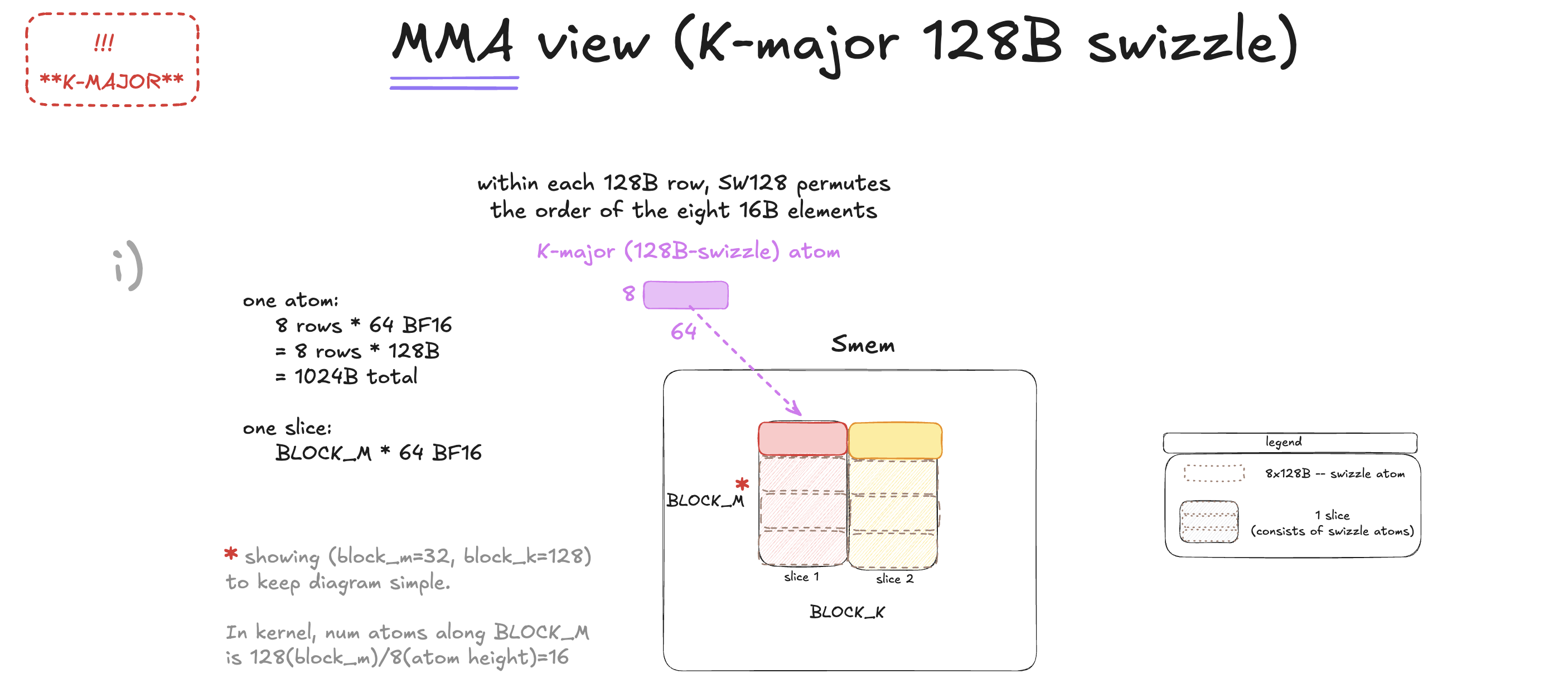
Now let’s zoom into what one of these 64-wide slices consists of.
One K-major SW128 atom is (8,64) BF16 (1024B).
One 64-wide Q slice consists of these atoms stacked along BLOCK_M.
Minor note, here I draw BLOCK_M=32 only to keep it readable; the real kernel has 16 atoms in each slice.
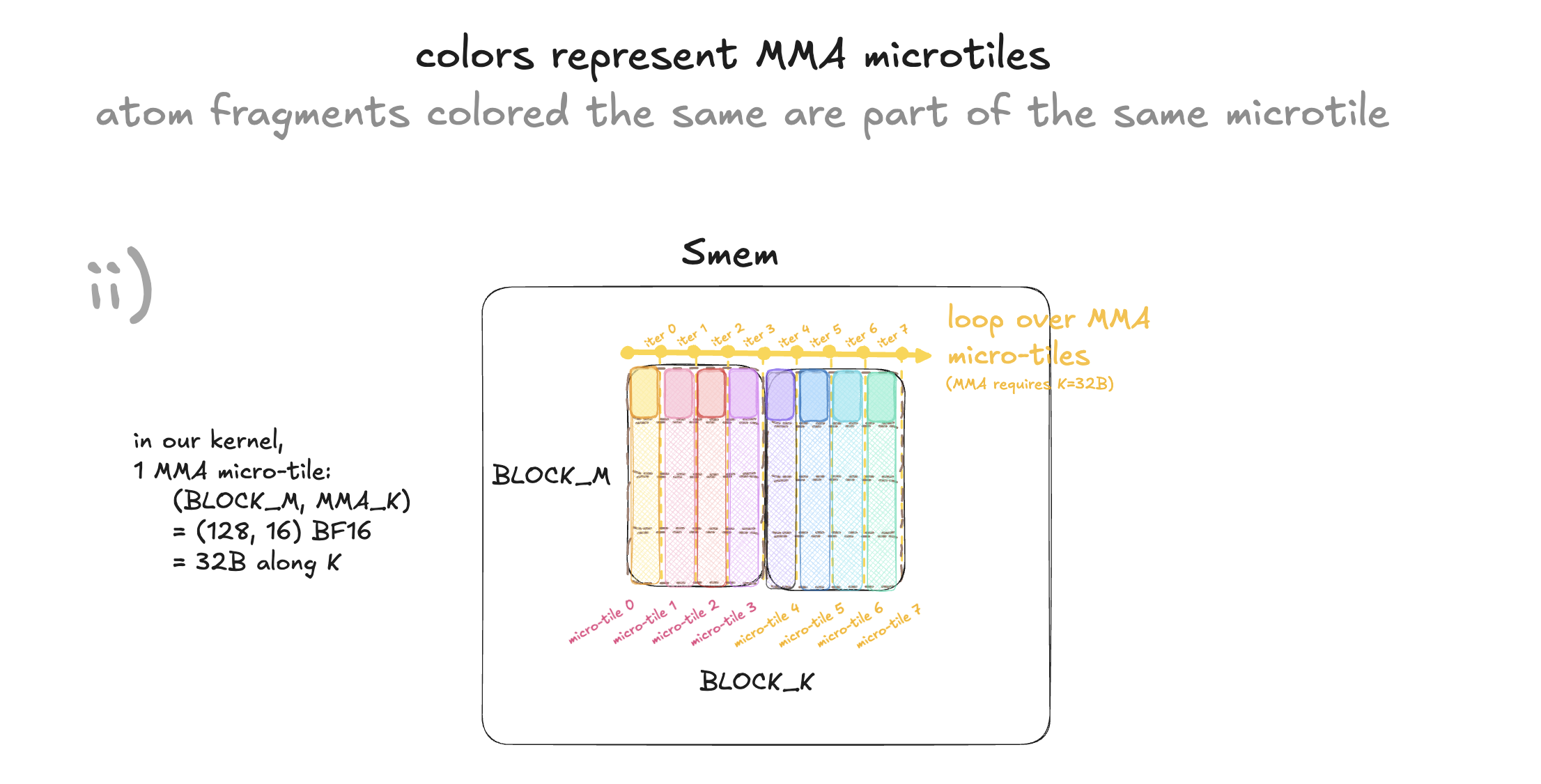
One MMA issue still operates on width MMA_K=32B (16 BF16 elements). But our BLOCK_K is larger than MMA_K, so (similarly as in no-swizzle case explained in ch1) we gonna need a for-loop which steps over BLOCK_K in MMA_K=16 element steps.
The difference here (compared to the non-swizzle case discussed earlier) is that logically,
now we gonna be splitting individual atoms, as each atom is of width=64, but MMA_K is only 16.
128B atom width / 32B mma width = 4 micro-tiles.
So whereas in the non-swizzle case we were taking 2 columns of atoms and calling it a micro tile, here our micro-tiles are result of splitting (and not combining) the atoms.
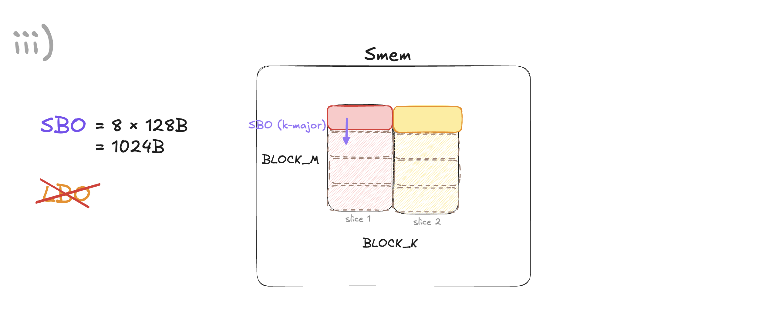
Inside one K-major SW128 slice, I think of SBO field as telling hardware how to reach the corresponding fragment in the next 8-row atom.
LBO is unused here, beucase as far as I understand:
- SBO already tells how to reach the other atom chunks in the same micro-tile, and separately,
- advancing the descriptor base(our software loop around MMAs) tells how to move to the next micro-tile. So these two together already cover both axis of the data.
So in this case, no additional offset (like LBO) is needed to specify another independent direction for stepping through the data.
To recap:
Once the major mode is chosen, SW128 tells us the shape of one atom and how its 16B elements are permuted inside it. But SW128 alone does not tell us the order of all atoms in the full tile.
Our TMA copy destinations decide where each atom lands in SMEM. On the MMA side, the descriptor base (which our software loop advances on each step over micro-tiles), and SBO, and if applicable LBO, must describe that same placement. Otherwise, tcgen05 will read the wrong data.
So far, we covered K-major layout with swizzling applied. Now let’s discuss the MN-major layout with swizzling applied, used for V in the PV matmul.
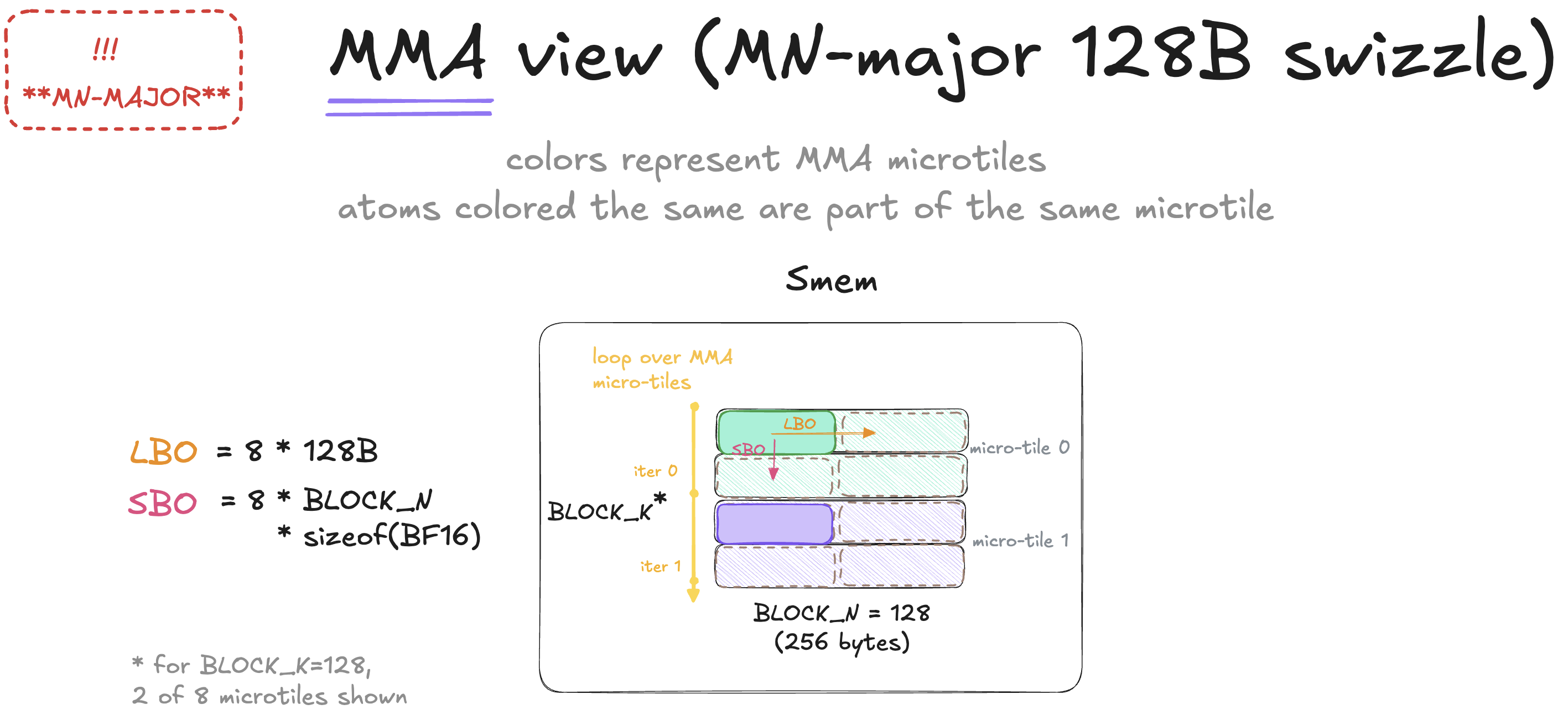
Each PV MMA microtile reads a 16×128 slice of V:
(16 rows along reduction-K and 128 columns along output-N).
Since each atom is 8×64, this slice contains four complete atoms.
In this V[K,N] view, LBO finds the next atom to the right,
while SBO finds the next 8-row stripe below.
The diagram shows two of the eight PV microtiles to keep it readable.
KERNEL CHECKPOINT
See 3_swizzle.cu and diff it against Kernel 2.
Now, familiarize yourself with the code.
Performance so far
| Kernel | Change | 4k | 8k | 16k |
|---|---|---|---|---|
| 1 | Baseline | 14.2% | 14.1% | 13.7% |
| 2 | P in TMEM | 15.1% | 15.0% | 15.0% |
| 3 | Swizzling | 25.9% | 25.9% | 26.2% |
Chapter 4 – Warp Specialization
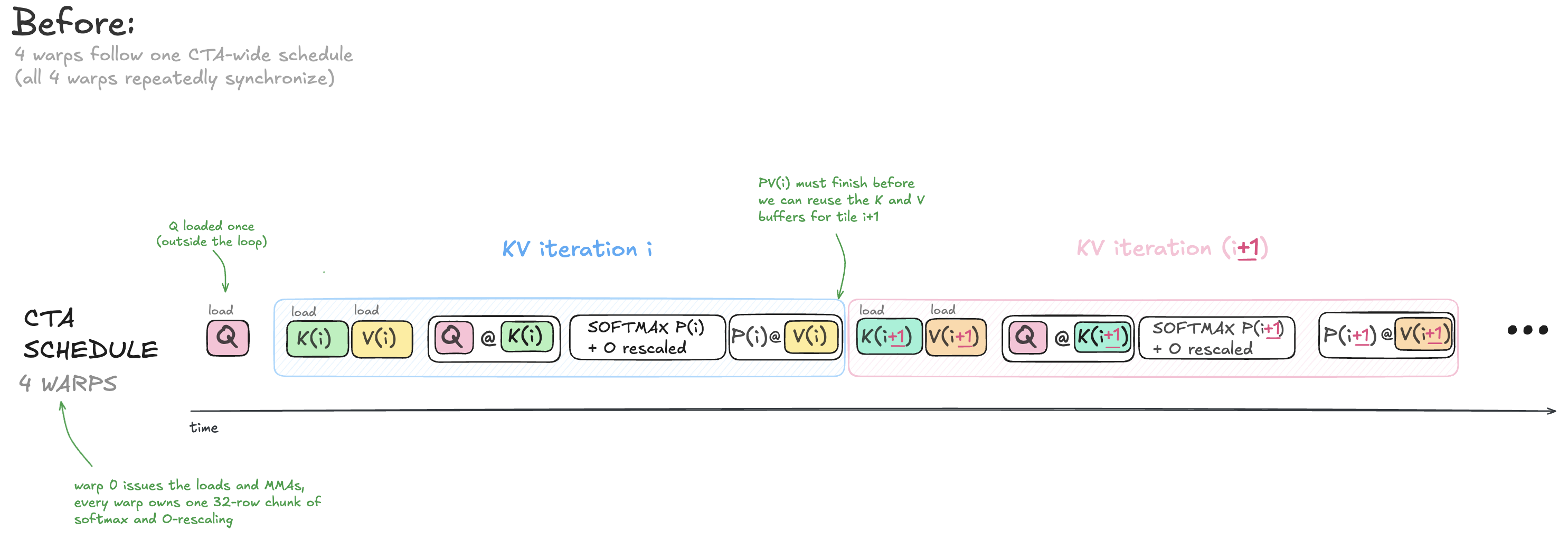
So far, our kernel uses 4 warps, each of which is independently schedulable.
But all of the 4 warps (128 threads) are synchronized multiple times throughout the kernel, so our synchronization is effectively CTA wide.
Earlier kernels already use mbarriers, which can be used more granularly,
but we still make all the warps wait on them, and several __syncthreads() calls still synchronize the entire CTA (as shown on the diagram above).
We would like to make workers (warps) independent so that later we can parallelize and overlap the work among them; but first we need to make the warps independent (not yet giving them independent work but sort of giving them capacity to run independently).
For example, if we have 128 threads total (4 warps), and at present we synchronize all of them at each arrow
load K/V(i) -> QK(i) -> softmax(i) -> PV(i) -> load K/V(i+1).
But we can rearrange our kernel in such a way that not all of the threads are synchronized at each arrow,
but only the ones which are need to synchronize for a given transaction (e.g. only 2 of the 4 warps can synchronize, without stalling the remaining 2 warps).
For example load producer and mma consumer handshake through a barrier, ie one producer warp arrives on the barrier signaling data is ready[^20], another consumer warp waits on the barrier, while other 2 warps don’t need to participate in the handshake, so in the future they can progress chugging along with their own work, without being stalled on a global handshake. This allows other warps (which are not needed for the transaction) to not be blocked/synchronized by it, and therefore to not pause their work unnecessarily.
Kernel 4 does that kind of transformation. Instead of synchronizing all 128 threads at every stage of the work (as in earlier kenels), we give each warp it’s work and we synchronize only the subset of them, which is actually relevant for a given transaction.
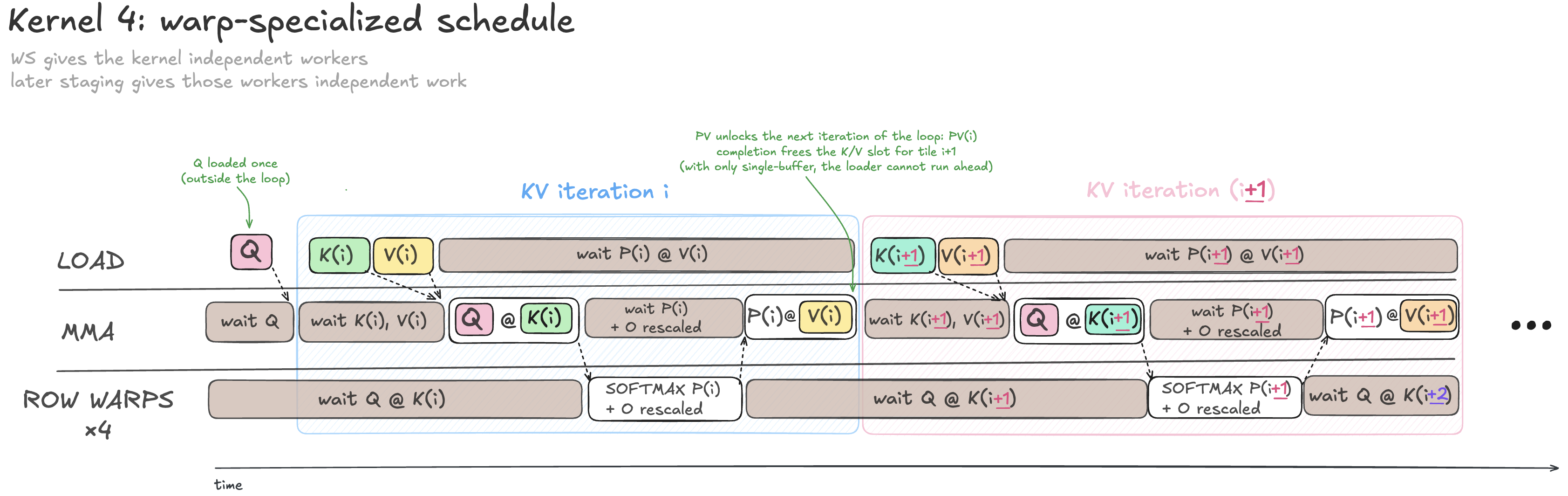
Notably, Kernel 4 gives warps independent roles, but it does not give them enough independent work to overlap yet. Ie the warps that don’t participate in a given handshake don’t overlap their own independent work yet – that’s what some of my later chapters do. So even though the warp roles now have separate instruction streams and the hardware operations are asynchronous, the major stages are still effectively serialized (load -> MMA -> softmax -> MMA). Concretely, for my earlier example of load warp and mma warp handshake, for now the rowwarps don’t have outstanding work to do so they are still sitting idle even though they don’t participate in the load-mma handshake directly.
This is clearly suboptimal (we’ll want to give these idle warps some work) and the topic of some of the future chapters. Which I did for teachability, rather than throwing all optimizations at once, so it’s easier to follow.
And this change alone is not expected to increase perf (it does not create more parallel work yet), but it enables our future optimizations. So basically, kernel 4 conceptually splits the kernel on individual workers, (where some do syncrize, but others now have the capacity to progress independently), and subsequent kernels given these workers independent work, turning that capacity into actual work overlap.
To create these independent workers, kernel 4 needs more warps than the previous kernel:
First, we’ll need 4 warps only for parallel processing of entire S->P the TMEM (because we have 128x128 S, and a single warp can only load 32-rows at a time, we want to load and process all 128 rows in parallel, thus we’d need 4 warps) and this will be our “row warps” – tasked with doing softmax, and O-rescaling.11
Second, if want want load warps be independent worker, we need one warp for that (cos the SMs scheduling granularity is in warps and not individual threads – so even though load worker only needs a single warp to launch TMA, we will allocate whole warp for it) so we have 5 warps at this point.
Then if want MMA to be a separate worker we need a separate warp for that also (by same the logic as in the TMA case above) resulting in 6 warps total.
So kernel 4 uses 6 warps in total: 4 row warps, 1 load warp, 1 MMA warp.
KERNEL CHECKPOINT
See 4_warp_specialization.cu and diff it against Kernel 3.
Now, familiarize yourself with the code.
Performance so far
| Kernel | Change | 4k | 8k | 16k |
|---|---|---|---|---|
| 1 | Baseline | 14.2% | 14.1% | 13.7% |
| 2 | P in TMEM | 15.1% | 15.0% | 15.0% |
| 3 | Swizzling | 25.9% | 25.9% | 26.2% |
| 4 | Warp specialization | 26.6% | 26.4% | 26.5% |
Part II — Coarse Scheduling
Chapter 5 – Two Q Tiles
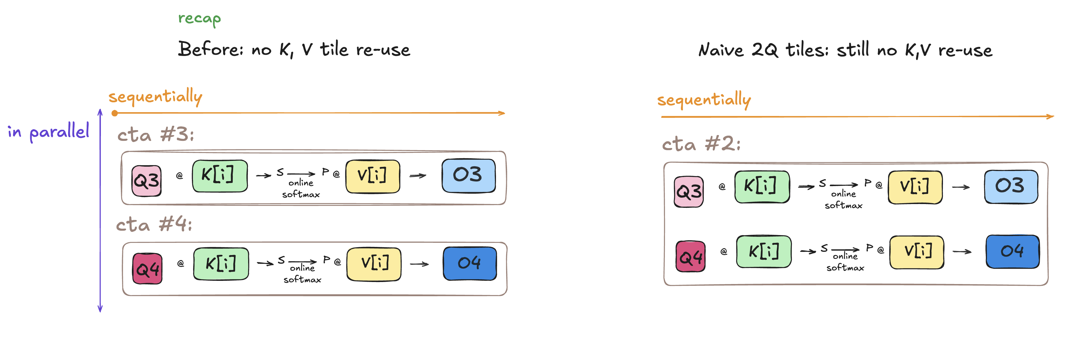
Kernel 4 assigns one Q tile to each CTA. So, two neighboring CTAs (ie CTAs which are assigned consecutive Q tiles for the same batch/head) independently loop over the same K/V tiles sequence and each of the CTAs loads the same K/V tiles. Though these are the same K and V operands which each CTA loads, so we can avoid loading them twice (once per Q tile / CTA) and instead re-use them (in each kv-loop iteration in a single CTA). Our next optimization is to let one CTA process two Q tiles and reuse each loaded K/V tile for both of them. This amortizes each K/V load across two Q tiles worth of work.
Simply moving both Q tiles into one CTA (left on the diagram above) is not enough. If we naively make one CTA process two Q/Output tiles, it wouldn’t create direct SMEM K,V re-use (if a CTA completes the entire KV loop for the first Q tile and then repeats the loop for the second, it still loads the same K/V tiles twice).
Kernel 5 instead loops over K/V once, using each loaded tile for both Q tiles.
load Q0 and Q1 once

for each KV tile i:
    load once K(i) and V(i)

    use K(i) for Q0K(i) and Q1K(i)
    use V(i) for P0V(i) and P1V(i)
For the same 2 Q tiles, this reduces the number of issued K/V TMA loads by half compared to our earlier kernels. We reuse the same KV tiles directly from SMEM (not L2 re-use: we’re not relying on the data staying in L2 across separate CTAs).
In the notation below, 0/1 identifies the Q stage, while i identifies the K/V tile, for example:
Q0K(i) = Q0 @ K(i)^T, and P0V(i) = P0(i) @ V(i). We will also use this naming convention for future kernels.
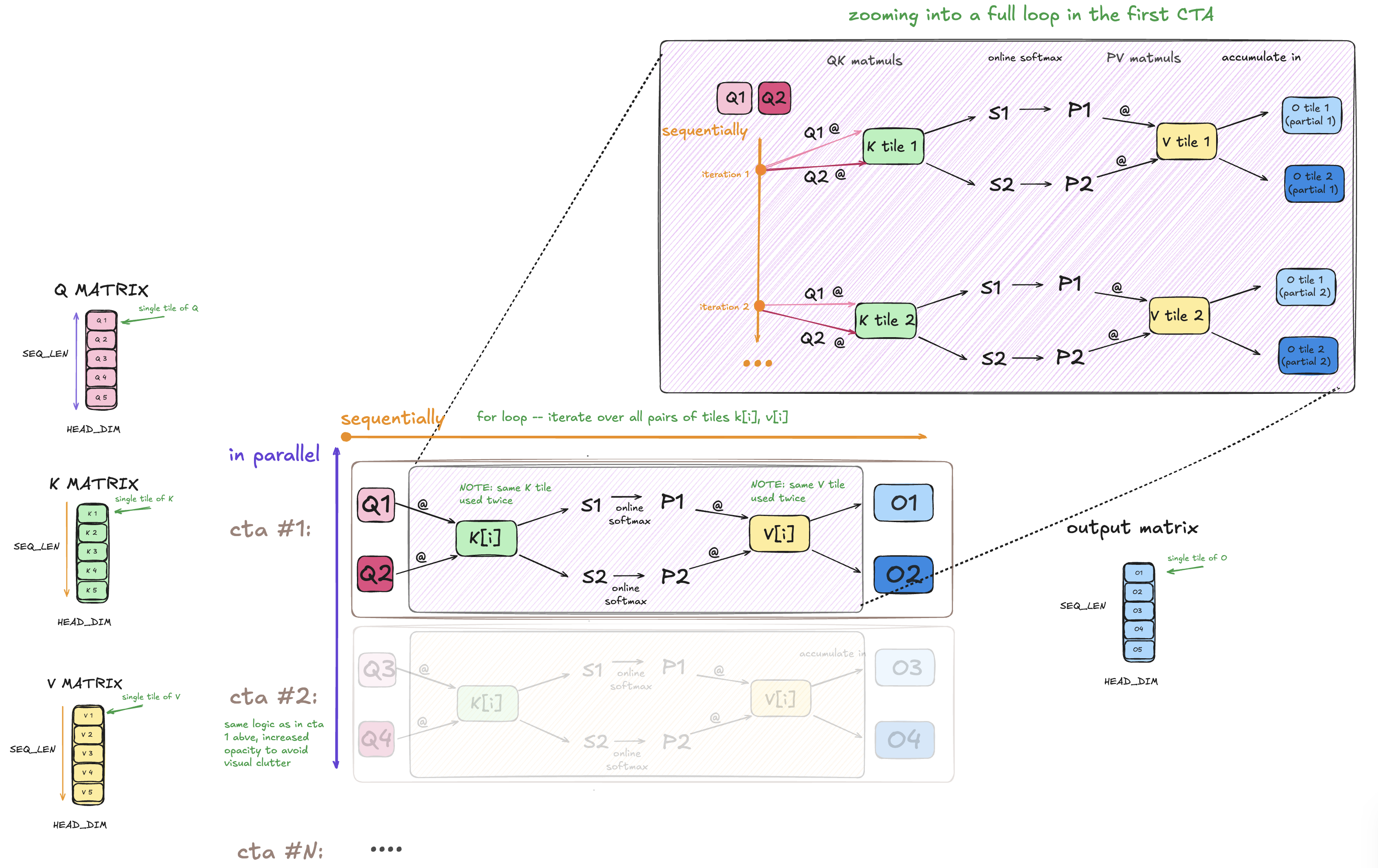
One CTA now owns two consecutive Q/O tiles of work (holds 2Q tiles for the duration of the kv-loop, and eventually produces 2-Output tiles).
Both Q stages reuse the same K/V tiles while they are still in SMEM, but QK, online softmax, and PV still run separately for each Q tile. Each Q stage keeps its own S/P tile, O accumulator, row maxes, and row sums.
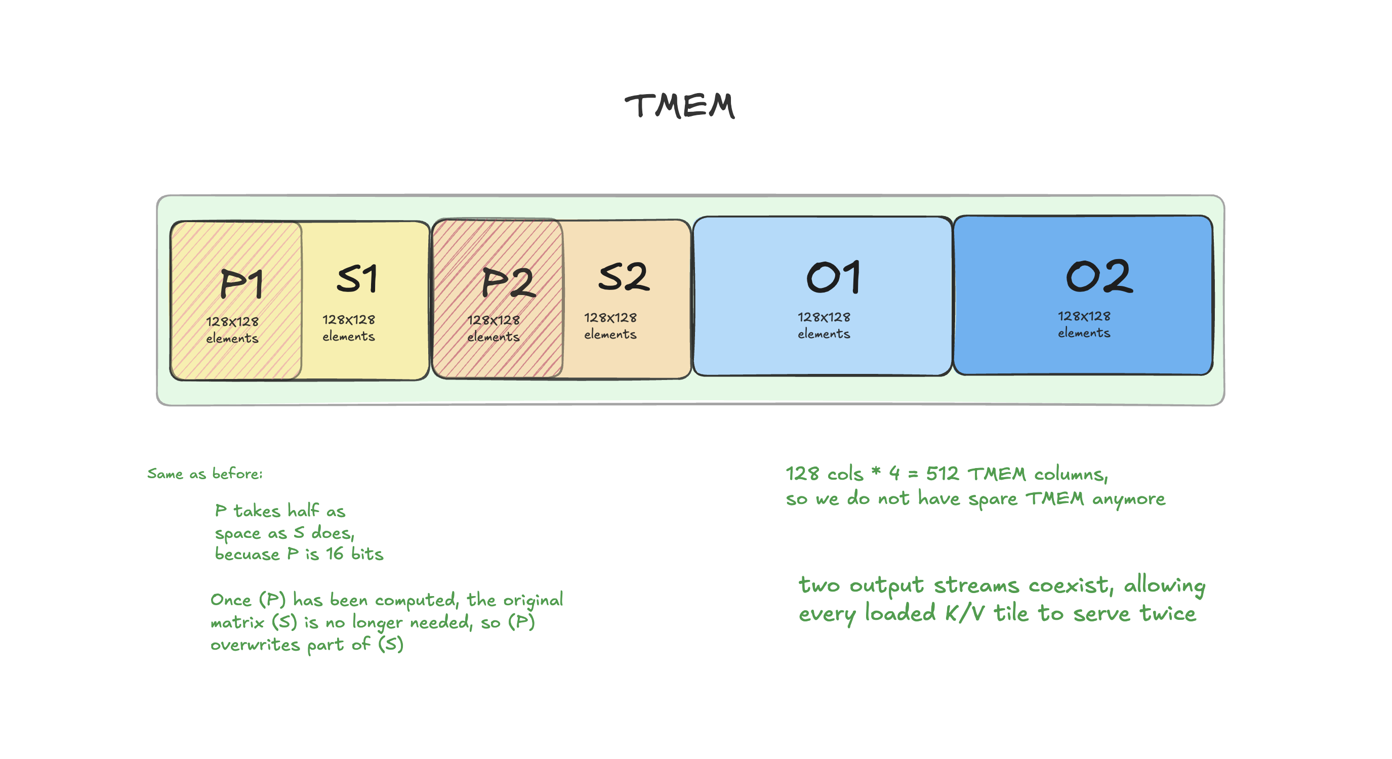
The second Q stream also needs its own TMEM state, so the layout becomes as illustrated above.
As before, each BF16 P tile consists of two packed values per each 32-bit TMEM cell and overwrites the lower half of it’s FP32 S allocation (as explained in Chapter 2). So, P0 doesn’t need additional storage beyond S0, and P1 doesn’t need additional storage beyond S1. This relies on the Chapter 2 change: if we didn’t write P into the dead-S’ buffer (and instead stored it in a separate TMEM region), we wouldn’t have enough TMEM to naively12 store S/P/O for two Q tiles.
Another angle to look at this optimization is: kernel 5 uses TMEM spatially (within the same KV-loop iteration), but not temporally (across KV-loop iterations). Meaning, two Q/Output streams are live at the same time and reuse K/V across the two live Q tiles (at the same KV-loop iteration), but not temporal compute pipelining (across different KV-loop iterations). All 512 TMEM columns are used, so there is no available TMEM to hold additional full stage S(i+1)/P(i+1) slots for future kv-loop iteration[s] on top of the two currently live Q-stage slots 13.
This does not implement load pipelining yet, Kernel 5 adds two-Q reuse, but it still has only one current K slot and one current V slot.
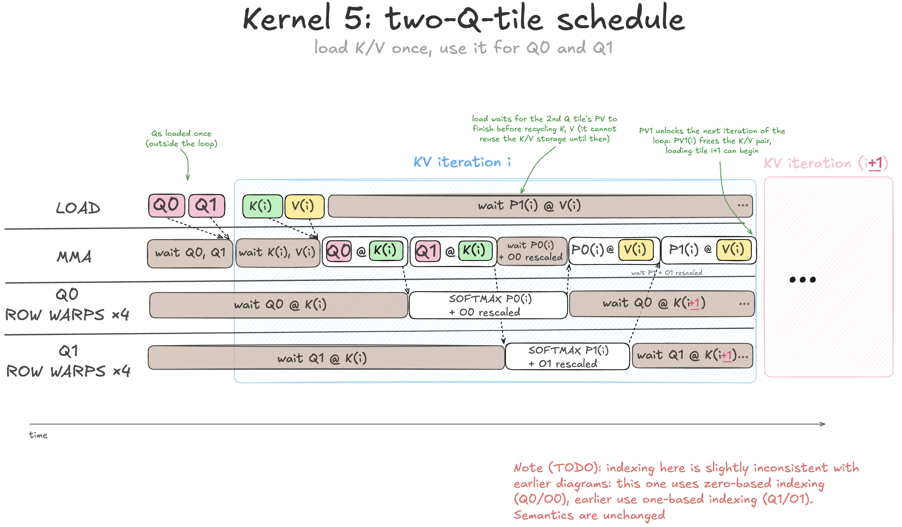
Previsoly we had 6 warps (see chapter 4), now the CTA has 10 warps:
warps 0..3:     row/softmax work for Q0
warps 4..7:     row/softmax work for Q1
warp 8:         TMA loads
warp 9:         QK and PV MMA issue
The two row-warp groups are independent: Q0 row work can start while the MMA warp processes Q1K.
Minor note on naming, I call them row warps and not softmax warps because these warps don’t just do softmax, but also O-rescaling (the same naming was used for chapter 4, so this is not new).
There is still only one MMA warp though, so Q0K, Q1K, P0V, and P1V are being issued by one ordered MMA stream rather than two parallel tensor-core streams. Adding another MMA warp would not create additional hardware tnesor-core pipeline because both target the same tensor-core hardware.
And tcgen05.mma is asynchronous, one issuer (selected lane) is enough to submit the MMA work. Instead, the bottleneck generally occurs when the MMA stream has no MMA to issue, for example operand is not ready. So the question is not whether we have another MMA warp, it’s whether the schedule exposes enough work to keep existing tensor core pipeline busy (creates operands fast enough so that MMA is not stalling for work; and MMA issue order doesn’t unnecessarily block MMAs from being issued on existing operands). Later optimizations address this by improving operand readiness and the schedule, not by adding another MMA issuer. That’s why we don’t add another MMA warp here, and keep only 1 MMA warp for the rest of the lineage.
As we added 2Q stages, this required adding new barriers. Some of the added barriers are shared by both Q stages, while others are separate for each stage:
- q_ready, kv_ready: shared by both Q stages. q_ready is used once before the KV loop starts; kv_ready is reused once per KV iteration.
- qk_done[q], softmax_done[q], pv_done[q]: separate stream for each Q stage
Each softmax_done[q] expects 4 arrivals, one for every row warp assigned to that Q stage. These row warps do both softmax/P production and O rescaling. Once all 4 arrived, it signals the P tile is ready and the old O accumulator is safe for PV. So this barrier represents both P ready and O-safe. MMA waits on this barrier before issuing PV.
As explained in the figure, becuase the K/V operands are now shared between two Q/O work items, we must ensure both of them finished using these buffers before re-using them for the next K/V tiles. So we re-use K/V storage only after P1V completes.14
KERNEL CHECKPOINT
See 5_two_q_tiles.cu and diff it against Kernel 4.
It follows the same optimizations we discussed.
Now, familiarize yourself with the code.
Performance so far
| Kernel | Change | 4k | 8k | 16k |
|---|---|---|---|---|
| 1 | Baseline | 14.2% | 14.1% | 13.7% |
| 2 | P in TMEM | 15.1% | 15.0% | 15.0% |
| 3 | Swizzling | 25.9% | 25.9% | 26.2% |
| 4 | Warp specialization | 26.6% | 26.4% | 26.5% |
| 5 | Two Q tiles | 40.5% | 40.3% | 41.3% |
Chapter 6 – Load Pipeline
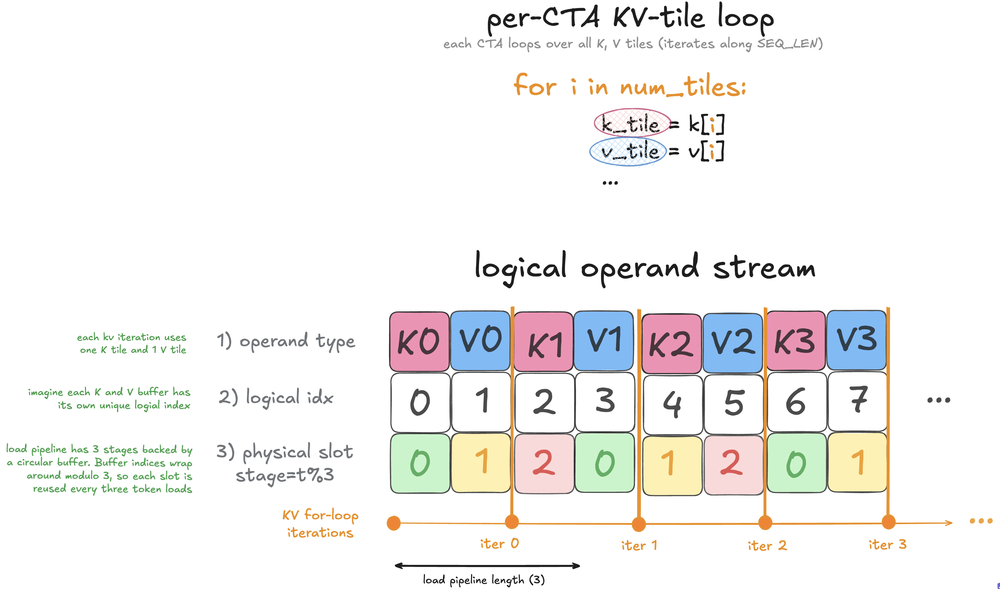
Don’t try to parse the diagram above yet, follow the text for now, I will draw your attention to the diagram later when needed.
So far, when we load K(i),V(i) tiles at each iteration of the loop, we stall and MMA warp waits until both are loaded. Only then QK can proceed, so the rest of the work downstream of QK (S->P, and eventually PV) is also blocked until both K and V operands are loaded.
There are two obvious inefficiencies there:
QKs only need K tile (Q@K needs no V tile) – so we can cut our load waiting time by letting QK proceed after only K is loaded (without waiting for V). This also unlocks work downstream of QK (S->P), and lets softmax begin earlier (less time idle).
We can significantly reduce idle time waiting for individual K/V loads, by pipelining the loads.
The second change is the main optimization of this chapter:
I like to think about this as producer (load warp) and consumer (mma warp), the idea behind pipelining is producer loading operands ahead of what the consumer needs. This way, the load generally has enough time to finish before the consumer needs it. When the consumer finally rolls around to that operand, it’s likely already loaded so MMA can just use it avoiding the stall. And when a future K or V operand is being loaded asynchronously, the consumer is busy working on operands already loaded in SMEM. This way we overalp load and compute.
The first change makes the pipeline finer grained:
We’re treating individual K or V as seprate operands being pipelined,
instead of treating K(i) and V(i) as one pair, which would require larger physical SMEM buffers. 15
Each of the 3 physical pipeline slots holds one K or one V tile.
KV[3] is one shared 3 slot pipeline buffer, and any slot may hold either K or V.
So, K and V are separated logically, but not placed in separate pipelines.
This lets the load warp run ahead instead of waiting for an entire K/V pair to become reusable.
This also relies on Chapter 2’s optimization, P no longer occupies K’s SMEM storage. K can therefore be recycled after QK while P remains alive in TMEM for PV.
In more details:
Q0 and Q1 are loaded once for the whole KV loop, so only the K/V operands (the ones which are changing each KV-loop iteration) participate in the pipeline.
Our load pipeline depth is 3 (3 physical buffers).
Before the KV loop begins, we pre-load K0, V0, and K1, filling all 3 pipeline buffers. K0 and V0 belong to the first KV-loop iteration, while K1 is loaded ahead for the next iteration. This preloads the data ahead of what the first consumer MMA will need (which is Q0@K0, Q0 is already loaded once before the for-loop, so K0 is the only operand), giving the producer a head start over the consumer.
In the for loop over KV tiles, each QK or PV uses a preloaded K or V operand, once the 2nd Q stage finishes using that operand, the corresponding consumer Q1K(i) or P1V(i) signals that the old token is no longer needed, the load warp, waiting in its own token loop, then re-uses that slot, issuing load for a future operand which is 3 (pipeline depth) logical positions ahead (now, please see the diagram ABOVE, it illustreate how it’s implemented in code).
With 3 token pipeline, there are 2 K/V tokens before the newly loaded token is needed. Each token is consumed by both Q stages, so MMA stream processes 4 full QK/PV matmuls before using the new token. This way a given load can be compleated in the background, and generally has enough time to finish loading that operand by the time the consumer needs it later. This effectively will overlap the load with compute.
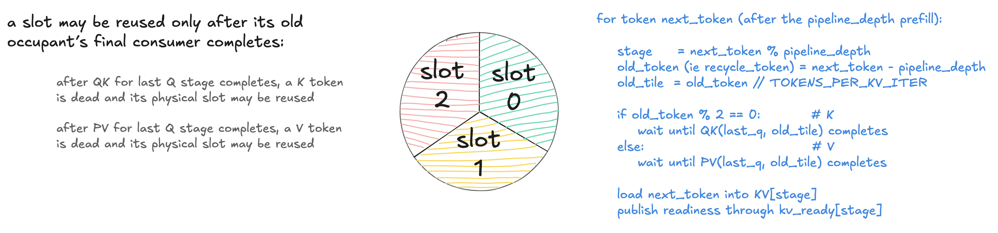
Of course in hardware buffer isn’t circular, but because the indices wrap around, and tokens separated by pipeline_depth (3) positions map to the same physical slot – it can be treated logically as a circular buffer. The data does not physically move around a circle.
Now covering both diagrams above, for this chapter, in more detail.
token identifies the logical K or V operand.
stage maps that operand onto one of 3 physical SMEM slots. It does not tell us whether that slot is ready or safe to overwrite.
Tokens t and t+3 use the same physical slot.
So, before loading token t, the loader must wait until the old token t-3 is used by its final consumer.
Because we have 2Q tiles and both Q0 and Q1 reuse the same K/V operand, we can recycle a given K or V token only after the last of the two Q tiles finished using it.
So:
- for a K token, the final consumer is the last-Q QK
- for a V token, the final consumer is the last-Q PV
Let’s see the logic behind the calculations we do on a concrete example (see diagram below):
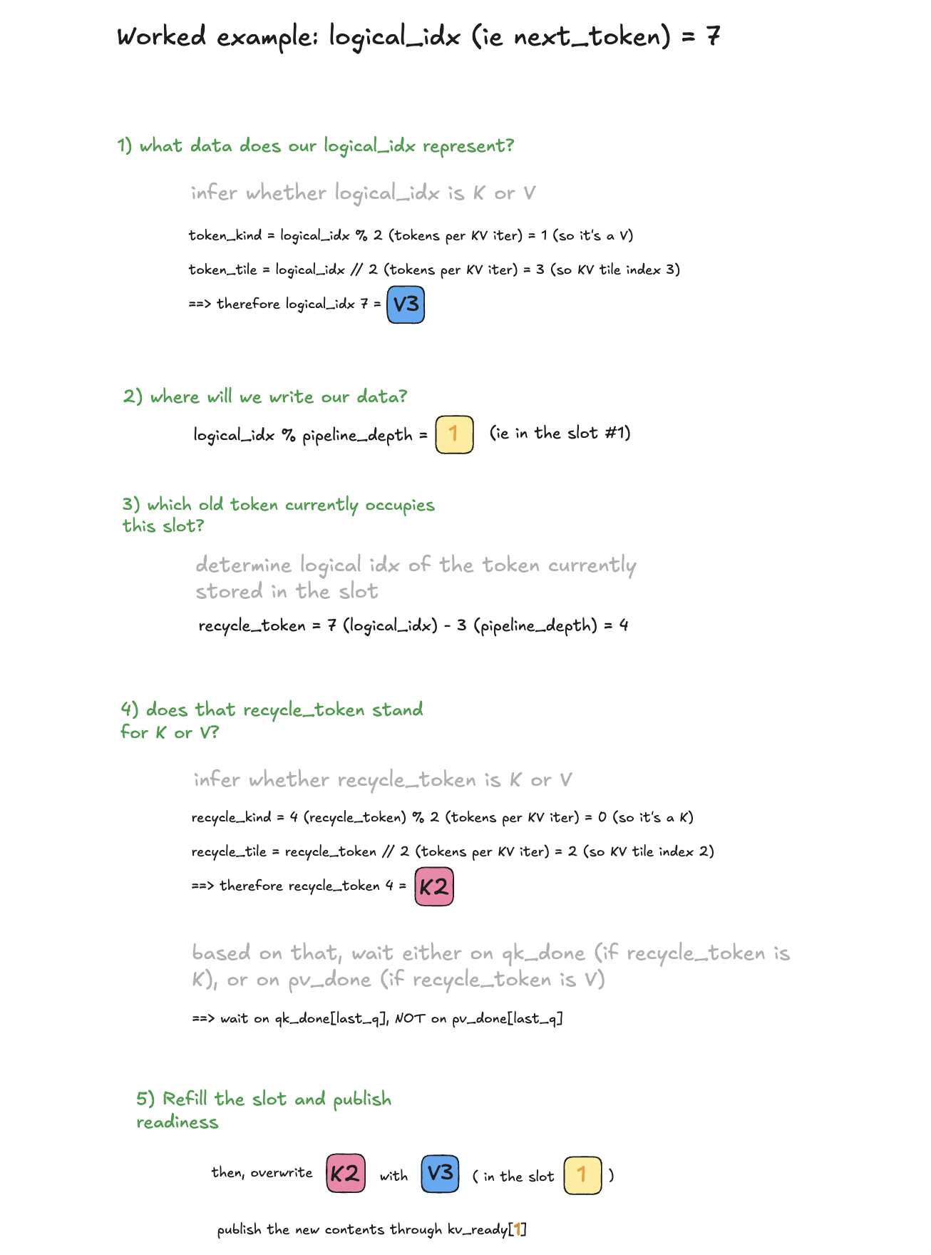
For a visualization of how the pipeline progresses (see the diagram below):
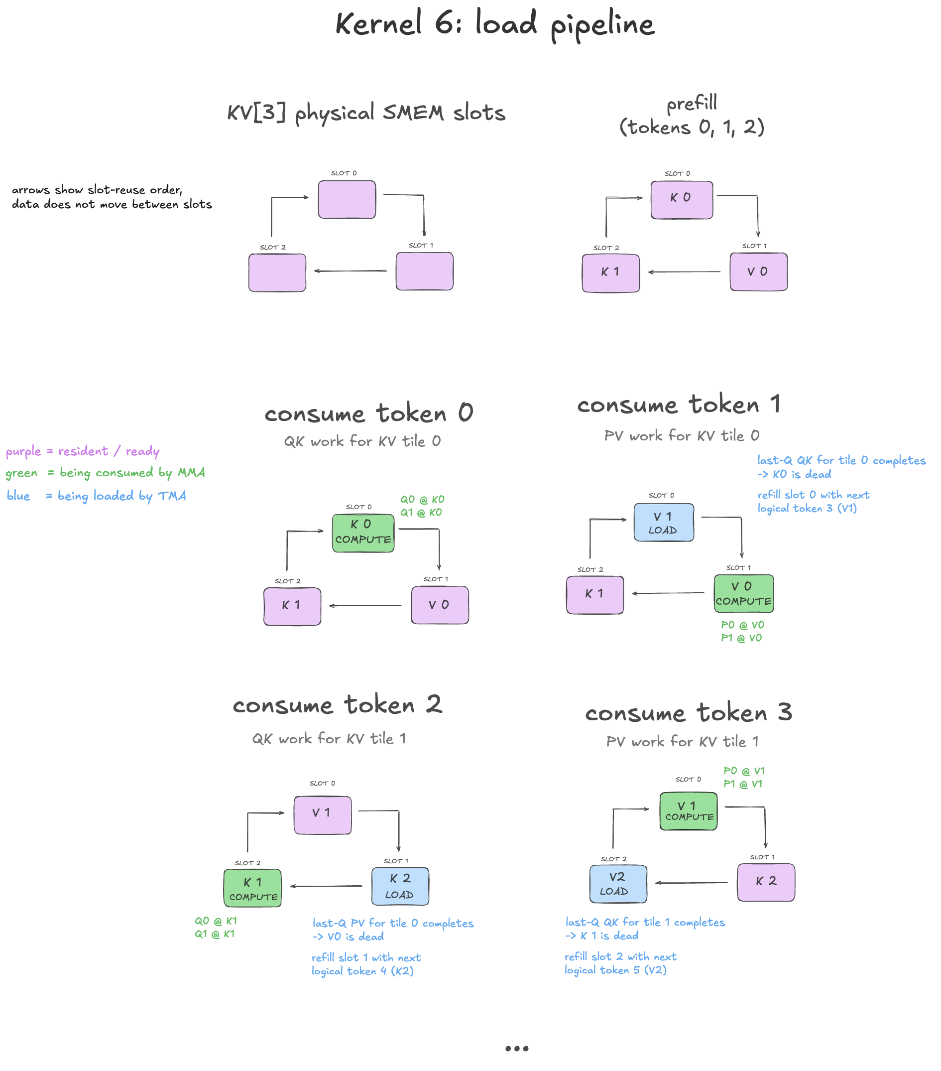
KERNEL CHECKPOINT
See 6_load_pipeline.cu and diff it against Kernel 5.
It follows the same optimizations we discussed.
Now, familiarize yourself with the code.
Performance so far
| Kernel | Change | 4k | 8k | 16k |
|---|---|---|---|---|
| 1 | Baseline | 14.2% | 14.1% | 13.7% |
| 2 | P in TMEM | 15.1% | 15.0% | 15.0% |
| 3 | Swizzling | 25.9% | 25.9% | 26.2% |
| 4 | Warp specialization | 26.6% | 26.4% | 26.5% |
| 5 | Two Q tiles | 40.5% | 40.3% | 41.3% |
| 6 | Load pipeline | 48.6% | 48.6% | 48.4% |
Chapter 7 – Compute Pipeline
Let’s recap the sheudle we have so far (in the earlier kernels), which is relevant for understanding our next optimization.
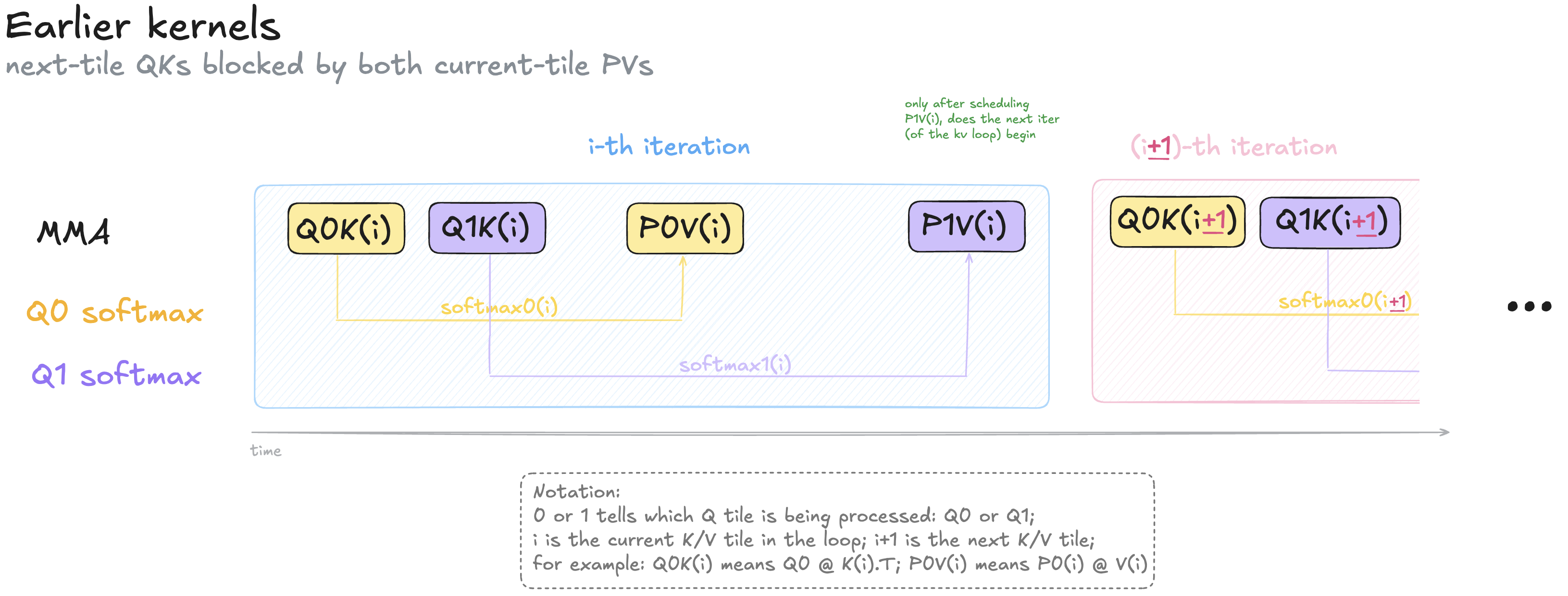
In our earlier kernels, MMA warp works on the granularity of kv-loop iterations, ie issues Q0K(i), Q1K(i), then P0V(i), P1V(i). And only then advances to the next kv-loop iteration.
So once PV for the 1st-Q-tile was issued, its row warps (softmax + O-rescaling) sit idle (unable to advance to the next kv-loop iteration) because the MMA warp does not reach Q0K(i+1) (ie 1st-Q-tile’ QK for the next iteration of the K/V loop) until after it issues 2nd-Q-tile’ PV.
This is clearly suboptimal, because 1st-Q-tile QK(i+1), and even more importantly its softmax(i+1) are blocked behind the 2nd-Q-tile PV(i).
Yet, as dicussed in the chapter 5 where we introduced the “2Q tiles” optimization, each of the 2 Q streams of work (which a given CTA processes) are mostly independant streams, with their own buffers (like S/P/O). They do share K/V, but that is not what forces Q0K(i+1) to wait behind P1V(i)16. So there’s no cross-Q-stage data dependency holding us from letting 1st-Q-tile to advance to the next kv-loop iteration (ie no dependency requiring Q0K(i+1) to remain behind P1V(i)).
Instead we want to issue 1st-Q-tile QK(i+1) and later its softmax work, as soon as 1st-Q-tile PV(i) is issued. This will allow the 1st-Q-tile softmax(i+1) to overlap with 2nd-Q-tile PV(i), which is highly desirable because as I said in the first chapter, the main bottleneck of this entire kernel is softmax work so the more of it we can overlap with MMAs the better.
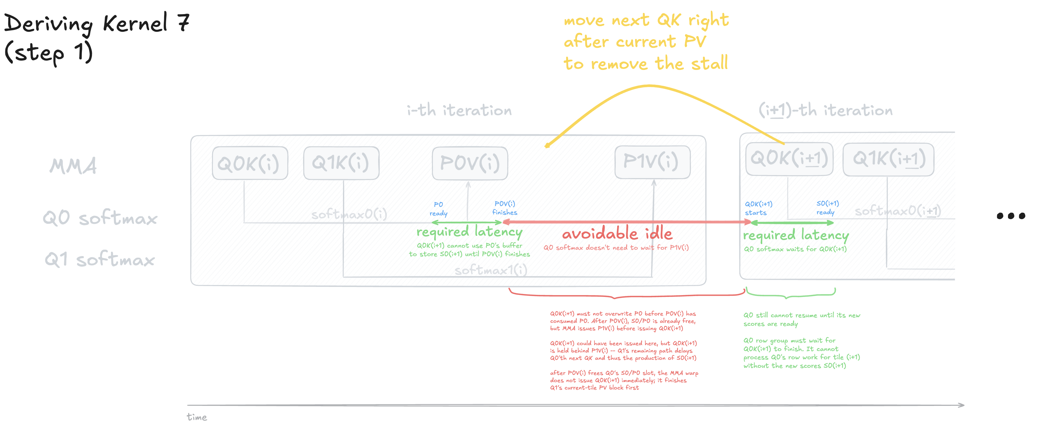
For the 1st Q stage, if we simply move its QK(i+1) to right after its PV(i) in the MMA schedule (once K(i+1) is ready), conceptually, we’ll achieve our desired result of unblocking this Q stage’s stream of work, letting it proceed to its next QK without being blocked by the 2nd-Q-tile PV.
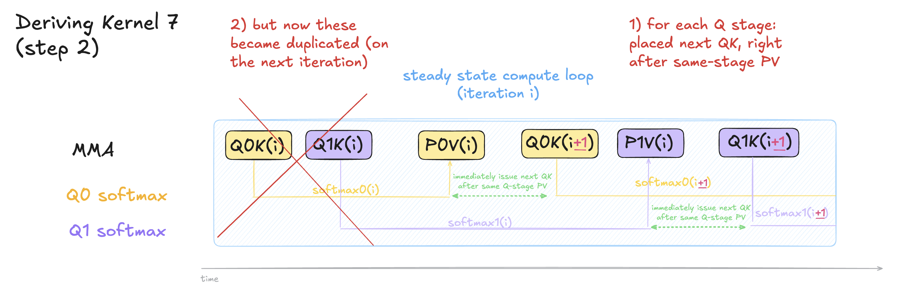
But notice if we naively move 1st Q stage’s QK(i+1) to the i-th iteration of the kv-loop, we would accidentally issue the same Q0K(i+1) twice: once near the end of iteration i, and again at the beginning of iteration i+1. And similar problem for the 2nd Q stage.
So there’s a few modifications we need to do to the kernel, discussed below.
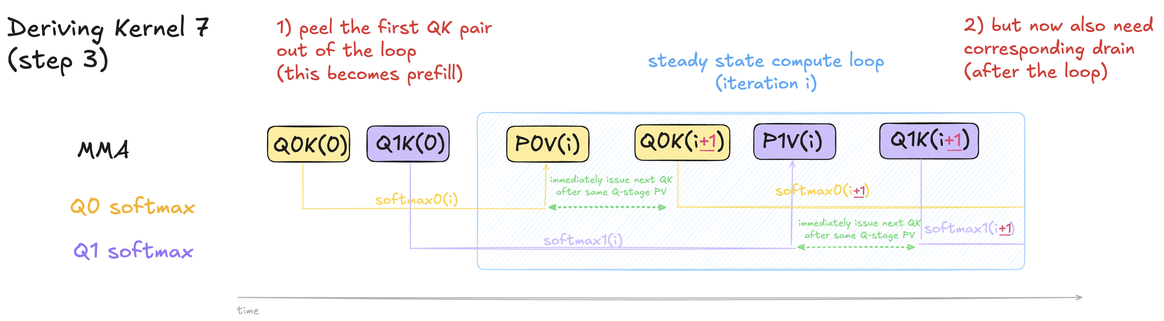
So we peel-off first QK (for each of Q stage) out of the for loop. Analogous to prefilling load pipeline as we done in kernel 6, but now we’re sort of prefilling the compute pipeline.
Now in the steady state of the loop we no longer issue the same next-tile QKs twice.
But as a consequence of the prefill before the loop, we also need a corresponding drain logically after the steady state loop (to exhaust the two Q stages work streams, because at the end of the loop over kv tiles there’s no subsequent iteration so unelss we add a drain, the final two PV tiles will not be executed).
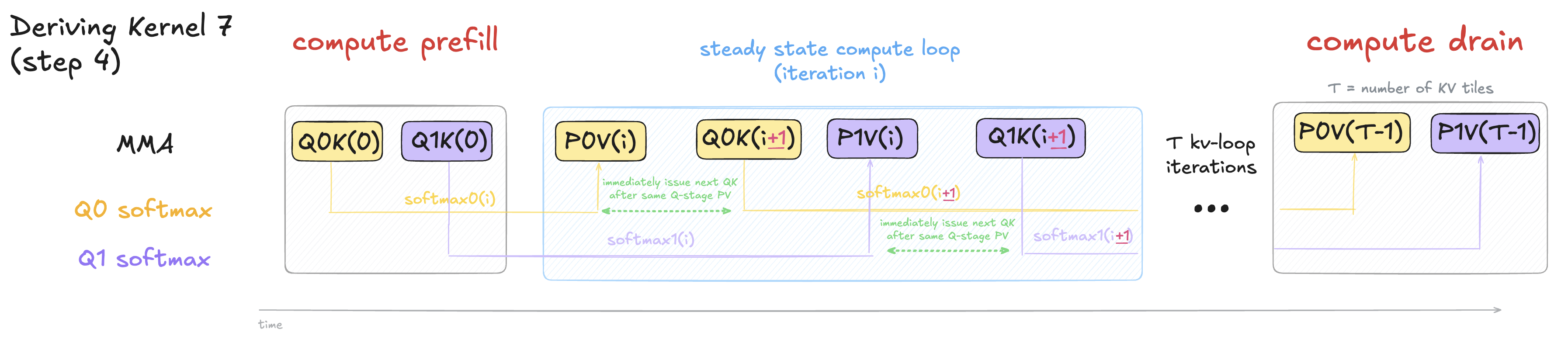
And that’s how we arrived to our final design for this chapter.
The schedule visually looks like we reversed QK and PV, but this is not the case. Here q is the Q-stage index (0 or 1). In the steady state, each loop iteration now finishes the current KV tile with PqV(i) and then starts the next KV tile with QqK(i+1). For any individual KV tile, the order remains QqK(i) -> softmax-q(i) -> PqV(i). So it only looks like we reversed QK and PV (for each Q tile), but we only moved the loop boundary; within each KV tile, nothing is reversed.
KERNEL CHECKPOINT
See 7_compute_pipeline.cu and diff it against Kernel 6.
It follows the same optimizations we discussed.
Now, familiarize yourself with the code.
Performance so far
| Kernel | Change | 4k | 8k | 16k |
|---|---|---|---|---|
| 1 | Baseline | 14.2% | 14.1% | 13.7% |
| 2 | P in TMEM | 15.1% | 15.0% | 15.0% |
| 3 | Swizzling | 25.9% | 25.9% | 26.2% |
| 4 | Warp specialization | 26.6% | 26.4% | 26.5% |
| 5 | Two Q tiles | 40.5% | 40.3% | 41.3% |
| 6 | Load pipeline | 48.6% | 48.6% | 48.4% |
| 7 | Compute pipeline | 58.2% | 58.5% | 58.0% |
Part III — Hot-Loop Optimizations
Chapter 8 – Hardware Approximations
This chapter doesn’t have anything meaningful for me to draw, so we’ll go over a little pseudocode instead. In chapter 10 we will continue with diagrams again.
So far, most of our optimizations changed the schedule. But the row-side softmax work is still the main bottleneck: this exp (part of S->P logic) runs per Q stage, per KV tile, per row, per 8-score chunk, which is what PV waits on. Extra work here gates the tensor cores. Our next few kernels (including Kernel 8) start making that hot path cheaper. So basically, we want to make the exp in our softmax hot path faster.
The GPU provides an approximate base-2 exponential instruction ex2.approx.ftz.f32.
The “approximation” in the name of this chapter, comes from the hardware computing exp2 approximately 17.
So, to try to speedup our hot path, we can use this instruction (hardware approximation)
instead of our __expf intrinsic we’ve been using.
But our online softmax still needs exp (and not exp2), while the hardware instruction computes exp2.
To produce the same value as regular exp would, we express the exponent in base-2,
using basically a math formula exp(x) = exp2(x * log2(e)).
So if we convert the input into the units expected by exp2 (by multiplying the input we’ve been feeding to exp by log2(e)),
its result is already the exp(x) value we need.
This identity itself is exact.
Actually … it turns out, __expf intrinsic we’ve been using in all our previous
kernels already lowers to ex2.approx.ftz.f32
(plus some wrapper instructions discussed later) !!!
So turns out we unknowingly been using that all along!
So at first, this optimization (of using asm ex2.approx.ftz.f32 directly), introduced in this chapter, looks redundant.
But in fact it’s not redundant and actually helps improve our kernel perf about 10%.
This sounds contradictory: if we were already using MUFU.EX2, where does Kernel 8’s speedup come from?
First, I’ll give the punchline, and then we’ll undersntad this deeper.
Turns out yes, __expf lowers to the same MUFU.EX2 core as ex2.approx.ftz.f32,
but with additional conversion and underflow-handling code around it.
And removing this additional wrapper code is what helps us improve the perf.
Now when we got the high level idea, let’s understand deeper.
The compiler expands that __expf intrinsic into something like:
// natural-exp argument originally passed to __expf
// float x = s * softmax_scale - rowmax;

// convert into base-2 exponent expected by exp2
// (see the math identity dicussed above)
float u = x * LOG2_E;

bool small = u < -126.0f;

// preserve results that'd underflow
// inside FTZ exp2 instruction
if (small) {
    u *= 0.5f;
}

float y;
asm("ex2.approx.ftz.f32 %0, %1;" : "=f"(y) : "f"(u));

if (small) {
    y *= y;
}
So, __expf desugars into an ex2.approx.ftz.f32 core plus some wrapper code around it.
For our use case, that wrapper has two pieces of avoidable work in the hot loop:
- repeated conversion to the log2 basis
- underflow behavior preservation (comparison in the predicate)
The reason for that wrapper code in the first place, is that the compiler cannot
infer our larger semantics, so conservatively chooses to do this
conversion (to the log2 basis, which the exp2 expects) locally for every expf in our hot loop,
and the underflow-handling around the EX2 (ex2.approx.ftz.f32) core is also emitted for
every __expf in our hot loop, and this additional work takes a noticeable bite out of performance.
Kernel 8 keeps the same num of MUFU exponentials, but basically removes the whole __expf wrapper:
- hoist that repeated conversion (to the log2 basis) out the hot loop and fold it into the existing S-scale, and
- remove the underflow checks and instead rely on the FTZ.
Let’s cover each of the two points above in turn.
1. Hoist repeated conversion to log2 basis out of the hot loop
In earlier kernels, we express the softmax directly in terms of natural-exp:
p = __expf(s * softmax_scale - rowmax);.
The compiler handles each __expf call locally.
In the generated code, it does not globally rewrite our online-softmax so that its
exponent inputs remain in exp2-friendly units.
So, it repeats the conversion to the log2 basis for every value in the hot loop.
Kernel 8 does that rewrite manually:
// fold the usual 1/sqrt(HEAD_DIM) attention
// scale together with log2(e)
softmax_scale_log2 = softmax_scale * log2(e);
// call ex2.approx.ftz directly
// (not the __expf which would add the wrapper)
p = fast_exp2(
        // scale S by that scaling factor, which includes log2,
        // so now the inputs are in exp2 input-friendly units;
        // subtract rowmax as usual
        s * softmax_scale_log2 - rowmax
        );
rescale = fast_exp2(old_rowmax - new_rowmax);
Rowmax actually also need to be in log2 units.
Recall from chapter 1, our kernel does two passes over TMEM to convert S into P.
The first pass over S still finds the maximum of the raw S scores, this stays unchanged.
After the reduction, in kernel 8, we multiply that one scalar (max per row) by softmax_scale * log2(e), which puts rowmax directly into exp2-input units.
So both sides of the subtraction above are in the units exp2 expects:
score:  s * softmax_scale * log2(e)
rowmax: already stored in those same units
P, rowsum, and O are not stored in log2 space. Only rowmax and the scaled S (which is passed to exp2) use these units.
2) Remove underflow handling and rely on FTZ
Second, we remove __expf’s underflow handling. So we remove the comparison and branching logic.
This part, unlike the first part above, is a real numerical apprixmation.
When the result is smaller than the smallest FP32 number (subnormal values), __expf wrapper tries to
preserve it by computing exp2(u / 2) and then squaring the result.
The __expf wrapper always computes the predicate of the if/else branches, even when, for almost all cases, the S value is large enough so that the branching logic doesn’t apply – but we still always pay for that compare in the predicate.
To decide “is this input in the underflow range?” we had to actually do the comparison, there’s no way to
skip the check that determines whether the check’s consequences apply.
So this compare instruction runs on every __expf call regardless of the score values.
But these two predicated fixup multiplies only matter when the result of exp2 is below 2^-126 (smallest FP32 value).
So, Kernel 8 deliberately flushes subnormal P and rescale values to zero. We make a call that this is acceptable here. This is what compiler could not have done for us, because this is not semantics preserving modification, and compilers are conservative to make such kind of modifications.
Once we stop trying to preserve subnormal results, there is no fixup to select, so we can remove the predicate and comparison too.
Direct ex2.approx.ftz.f32 skips that handling and simply
turns the value into zero (denoted by the FTZ in the instruction name).
Together, these two choices let us remove the per-call __expf wrapper, its
base2-conversion, range check, and predicated underflow handling.
Official FA4 makes the same direct-FTZ choice.
SASS comparison:
MUFU.EX2:             129 -> 129
static instructions: 3296 -> 2776
predicated inst:       368 -> 110
FMUL:                   644 -> 257
FSETP.GEU.AND:          129 -> 0
So Kernel 8 changes didn’t reduce MUFU count, but made the work around each MUFU cheaper.
KERNEL CHECKPOINT
See 8_hardware_approx_exp2.cu and diff it against Kernel 7.
Now, familiarize yourself with the code.
Performance so far
| Kernel | Change | 4k | 8k | 16k |
|---|---|---|---|---|
| 1 | Baseline | 14.2% | 14.1% | 13.7% |
| 2 | P in TMEM | 15.1% | 15.0% | 15.0% |
| 3 | Swizzling | 25.9% | 25.9% | 26.2% |
| 4 | Warp specialization | 26.6% | 26.4% | 26.5% |
| 5 | Two Q tiles | 40.5% | 40.3% | 41.3% |
| 6 | Load pipeline | 48.6% | 48.6% | 48.4% |
| 7 | Compute pipeline | 58.2% | 58.5% | 58.0% |
| 8 | Hardware exp2 | 64.1% | 64.1% | 63.8% |
Chapter 9 – Software Approximations
This chapter doesn’t have anything meaningful for me to draw, so we’ll go over a little pseudocode instead. We will continue with diagrams in the next chapter.
Kernel 8 removed extra wrapper work around every hardware exponential,
but all P exponentials still went through the same MUFU.EX2 pipeline.
Kernel 9 moves some of these exponentials off MUFU and approximates them in software using regular ALU/FMA instructions.
So we do not reduce num of exp computations (we still need to exp each value in S, as in all our previous kernels). But now we speread the workload across two different pieces of hardware, reducing pressure on the MUFU pipeline.
The split is:
for each 16 P values:
    first 12 -> hardware exp2
    final 4  -> software exp2
Thus, 25% of the P exponentials use the software path. This selection depends only on the column position, not on the individual P values themselves.
The exact split (25% for ALU and 75% for MUFU) is determined experimentally, and is not a hard requirement. Software exp2 needs more instructions, temporary values, and registers. Moving everything to software would move the bottleneck onto other resources.
Why can several software instructions be faster than one hardware instruction? Because software exp2 uses different execution resources. The hardware path is shorter, but all those exponentials compete for the relatively limited MUFU pipeline. Moving some of them to the regular ALU pipelines gives GPU more independent resources with which to do the work.
SOFTWARE EXP2 WALKTHROUGH
Explanation above is enough to follow the rest of the blog.
For an optional walkthrough of the approximation math, see How Software exp2 Works in the Appendix.
The helper looks like:
float software_exp2_scalar(float x) {
    // polynomial coefficients
    float C3 = 0.077f;
    float C2 = 0.227f;
    float C1 = 0.695f;

    // input is in base-2 units, and we want to compute 2**x,
    // if x is below -127, that means 2**x will be extremely small,
    // so small that we don't care (FTZ like)
    x = fmaxf(x, -127.0f);

    int int_part = floor(x);
    float frac_part = x - int_part;

    // approximate 2^frac_part using three chained FMAs;
    // as an optimization, feed each result into the next FMA,
    // avoiding separate frac_part^2 and frac_part^3 computations
    float frac_exp2 = C3;
    frac_exp2 = fma(frac_exp2, frac_part, C2);
    frac_exp2 = fma(frac_exp2, frac_part, C1);
    frac_exp2 = fma(frac_exp2, frac_part, 1.0f);

    // expose the bits of our approximate 2^frac_part
    int frac_exp2_bits = __float_as_int(frac_exp2);

    // FP32 has 23 fraction bits, so 1 << 23 is one exponent step
    int exponent_adjustment = int_part * (1 << 23);

    // combine approximate 2^frac_part with 2^int_part
    int result_bits = frac_exp2_bits + exponent_adjustment;
    return __int_as_float(result_bits);
}
This algorithm is adapted from FA4’s ex2_emulation_2.
This is a simplified version, processes one value for clarity.
The actual helper
performs the same algorithm on two values together using packed f32x2 instructions.
Both paths (hardware exp2, added in chapter 8; and this chapter’s software exp) are approximate. This optimization changes only how selected P values are computed and does not reduce number of exp computations.
KERNEL CHECKPOINT
See 9_selective_software_approx_exp2.cu and diff it against Kernel 8.
Now, familiarize yourself with the code.
Performance so far
| Kernel | Change | 4k | 8k | 16k |
|---|---|---|---|---|
| 1 | Baseline | 14.2% | 14.1% | 13.7% |
| 2 | P in TMEM | 15.1% | 15.0% | 15.0% |
| 3 | Swizzling | 25.9% | 25.9% | 26.2% |
| 4 | Warp specialization | 26.6% | 26.4% | 26.5% |
| 5 | Two Q tiles | 40.5% | 40.3% | 41.3% |
| 6 | Load pipeline | 48.6% | 48.6% | 48.4% |
| 7 | Compute pipeline | 58.2% | 58.5% | 58.0% |
| 8 | Hardware exp2 | 64.1% | 64.1% | 63.8% |
| 9 | Software exp2 | 69.3% | 70.1% | 70.6% |
Chapter 10 – Register Caching
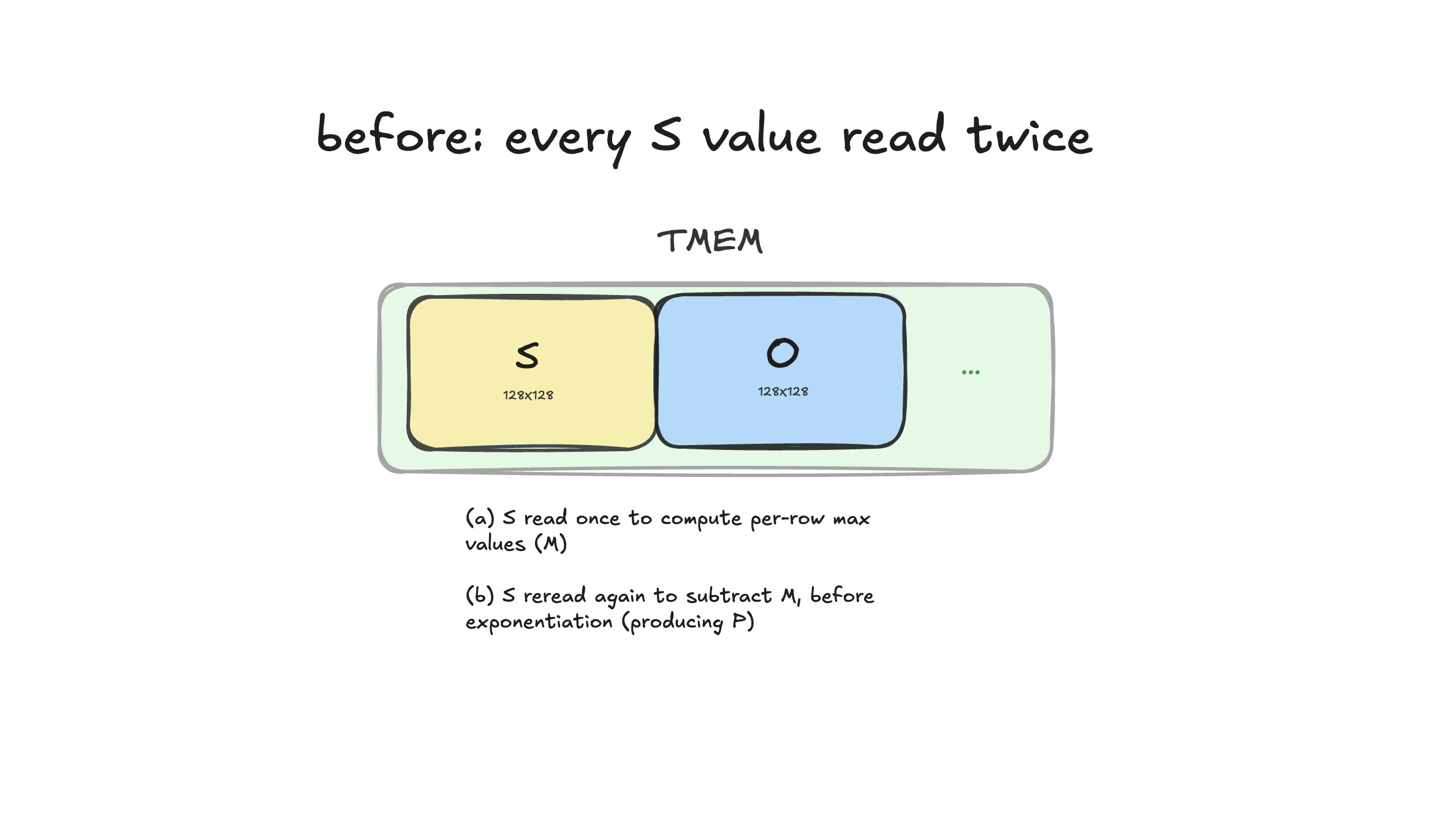
In the earlier kernels, for each Q stage, we traversed S in TMEM and read it twice (explained in chapter 1). First, to compute rowmaxes (to be used for numerical stability in the 2nd step). Second, to subtract rowmaxes and exponentiate the result (so we first need to have computed rowmaxes before we can subtract them in this step, which is why we traversed same S in the TMEM twice).
Our next optimization reduces 2nd-pass TMEM re-reads by retaining part of S in registers.
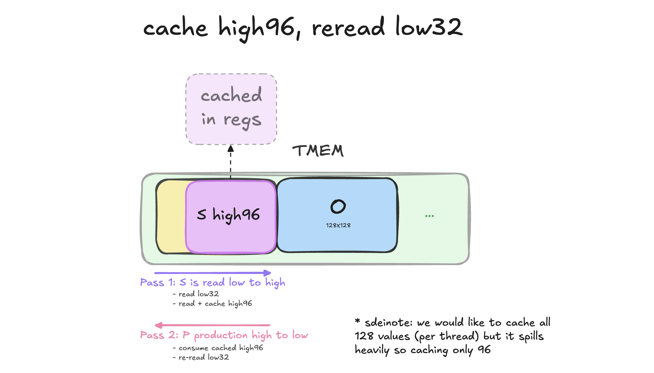
So we want to reduce register lifetimes, so we:
- (a) in the 1st pass over TMEM, cache the most recent values of S that we read (because we read S low to high, it’s the high 96 cols which we encountered latest)
- (b) change the P-production pass (previously the 2nd TMEM pass) to traverse high to low (so these recently cached values are consumed first)
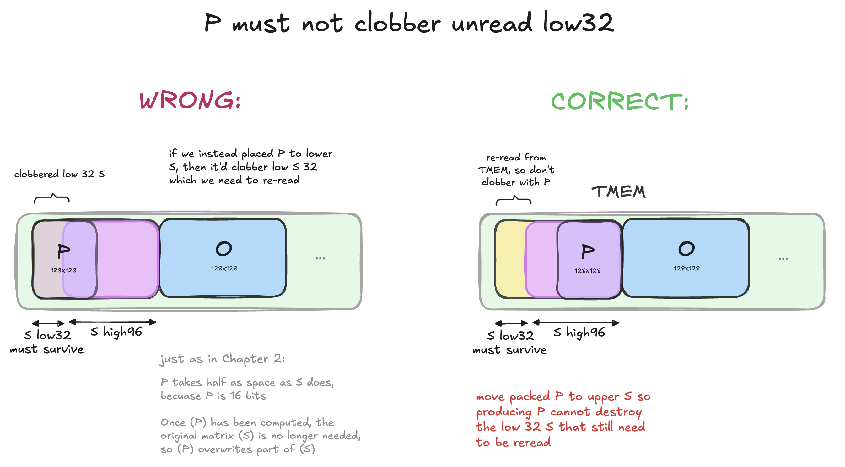
In the previous kernels (beginning from Chapter 2), we stored P in the lower part of S region in TMEM. In this chapter, since only the high 96 are cached (as explained earlier), the low 32 must be re-read later (128 cols total). So we cannot store the high 96 P at the lower S anymore (storing P at lower S, would clobber the low 32 S before that reread), so begining from Chapter 10, we store P at the upper half of S.
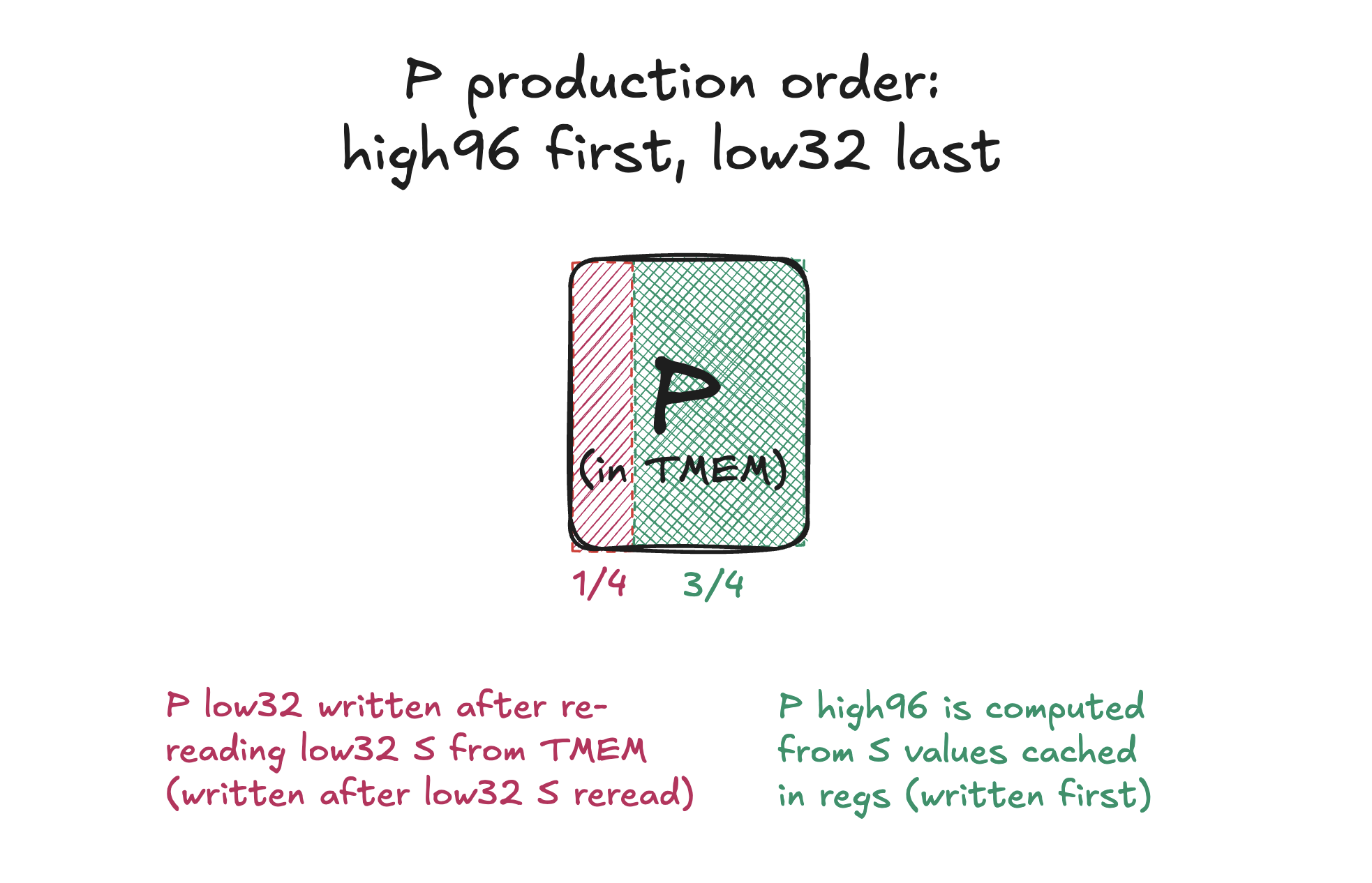
One more detail: the re-read S low32 are needed to produce only 1/4 of P. The rest 3/4 of P is produced using the S values cached in regs.
Therefore, the second pass over S remains, but it rereads only 32 of 128 scores from TMEM, removing 3/4 of the re-reads.
KERNEL CHECKPOINT
See 10_cache96_reread32.cu and diff it against Kernel 9.
Now, familiarize yourself with the code.
Performance so far
| Kernel | Change | 4k | 8k | 16k |
|---|---|---|---|---|
| 1 | Baseline | 14.2% | 14.1% | 13.7% |
| 2 | P in TMEM | 15.1% | 15.0% | 15.0% |
| 3 | Swizzling | 25.9% | 25.9% | 26.2% |
| 4 | Warp specialization | 26.6% | 26.4% | 26.5% |
| 5 | Two Q tiles | 40.5% | 40.3% | 41.3% |
| 6 | Load pipeline | 48.6% | 48.6% | 48.4% |
| 7 | Compute pipeline | 58.2% | 58.5% | 58.0% |
| 8 | Hardware exp2 | 64.1% | 64.1% | 63.8% |
| 9 | Software exp2 | 69.3% | 70.1% | 70.6% |
| 10 | Register caching | 72.9% | 73.7% | 73.6% |
Chapter 11 – Skip O rescale
This chapter doesn’t have anything meaningful for me to draw, so we’ll go over a little pseudocode instead. In the next chapter we will continue with the diagrams.
In regular softmax, we see the entire row, find the final rowmax once, subtract it, and then compute the exponentials.
Online softmax processes one K/V tile at a time, so we don’t know the final rowmax in advance, it discovers the row tile by tile, so a later tile may contain a larger maximum. So the unique decision online softmax has to make (unlike the reguaral full softmax) is:
- Do we immediately switch to every newer maximum?
- Or can we keep using the old rowmax?
In earlier kernels, whenever we found a larger maximum, we immediately started using it:
new_rowmax = max(old_rowmax, tile_rowmax)
Then they expressed all the old state in that new basis:
old O      *= rescale
old rowsum *= rescale
The rowsum update is cheap, but rescaling O requires another full traversal
of its 128 values per row in TMEM.
Kernel 10 ran this O pass after every iteration of the kv-loop, even when the scale was 1.
So, Kernel 10 traversed the entire O tile when the maximum did not change and rescale == 1.
So it loaded 128 O values, multiply them by one, and store them back.
That is numerically safe but unnecessarily conservative.
In Kernel 11, if the new tile maximum is only slightly above our currently kept rowmax, we keep using the old rowmax and leave O and rowsum unchanged. If the difference is large enough, only then we switch to the new rowmax and rescale the old O and rowsum into the new basis.
Skipping rescaling doesn’t erase information
This was not immediately obvisous to me18, but let’s see what happens when we skip rescaling O on a little example, to convince ourself that no information gets lost (as a reuslt of us skipping the rescale).
Suppose we decided to skip O rescale for a given tile
(we gonna discuss the specific threshold value later).
For now, let’s just say our current tile’s maximum is 7.78 above our old rowmax.
We still compute P relative to the old rowmax:
P = exp2(scaled_S - kept_rowmax)
So, the newer maximum produces:
exp2(7.78) ~= 219
So even though we skipped rescaling O, the newer maximum is not erased and no info is lost. Because we still compute P using the old rowmax, that larger score turns into an unnormalized P value about 219x as large. That larger P value is where the difference remains preserved.
Even better, compared to the world where choose to rescale instead, the final result of our entire kernel does not change at all. Because the larger P enters both parts of softmax, the larger P values enter both the numerator O and the denominator rowsum.
The same P values enter both parts of attention:
O      += P @ V
rowsum += sum(P)
So, for my earlier 219 example:
O      += 219 * V_new
rowsum += 219
Then, after the entire K/V loop:
output = O / rowsum
So the newer score is still treated as about 219x larger in both O and rowsum. The final division does not erase that 219x relative difference; it only cancels the common scale shared by O and rowsum.
Then why rebase at all?
If the final O / rowsum handles the common scale,
it seems like we could keep the first rowmax forever.
Mathematically seems, we can, as long as all the intermediate values don’t overflow.
For example, if the old rowmax became very stale:
gap = 20
largest P = exp2(20) = 1,048,576
The final answer will still mathematically be equivlant, but P, rowsum, and O would now use huge intermediate values. If these overflow, obviously the final normalization (dividing by the rowsums) cannot undo that overflow.
How the per-row decision maps to the warp-wide TMEM O pass
The decision to rebase is made separately for each row, but the TMEM O loads and stores are warp-collective. So the actual implementation looks like this:
// convert the current tile's raw rowmax into base-2 exponent units
tile_rowmax *= softmax_scale_log2;

// kept_rowmax is already stored in the same units
float candidate_rowmax = max(kept_rowmax, tile_rowmax);
float rowmax_gap = candidate_rowmax - kept_rowmax;
bool row_needs_rebase = rowmax_gap >= REBASE_THRESH_LOG2;

float rescale = 1.0f;

// 1) if needed, rescale this row's state and start using the new rowmax
if (row_needs_rebase) {
    // this factor will be applied to both rowsum and O
    rescale = fast_exp2(kept_rowmax - candidate_rowmax);

    // move this row's scalar accumulator into new rowmax basis
    rowsum *= rescale;

    // use new rowmax when producing this P tile and future P tiles
    kept_rowmax = candidate_rowmax;
}

// 2) apply same rescale factor to O
//
// TMEM loads/stores are warp-collective. If any row needs rescaling,
// entire warp must process its 32x128 O slab.
// Rows that don't rebase still participate but with rescale 1
if (__any_sync(FULL_WARP_MASK, row_needs_rebase)) {
    float o8[8];

    // same O traversal used in earlier kernels
    for (int col = 0; col < HEAD_DIM; col += 8) {
        int taddr = taddr_o_stage + trow + col;

        tcgen05::ld_32x32b_x8(taddr, o8);

        for (int i = 0; i < 8; ++i) {
            o8[i] *= rescale;
        }

        tcgen05::st_32x32b_x8(taddr, o8);
    }

    asm("tcgen05.wait::st...");
    asm("tcgen05.fence::before_thread_sync...");
}

// P production and the later PV proceed as in earlier kernels,
// using kept_rowmax as the rowmax for this tile
Actual thresh value
Since Kernel 8 we express our exponent inputs in base-2 units. Kernel 11 uses threshold of 8 base-2 exponent units, matching official FA4. As far as I understand, there is no deep mathematical cliff at 8. Larger thresholds such as 12 or 15 numerically plausible for our BF16-P/FP32-accumulator path. 8 is a conservative point that already appears to skip most useful O-rescale opportunities not an overflow boundary.
exp2(8) = 256
So we keep using the old rowmax while the largest unnormalized P value, computed relative to that rowmax, stays below roughly 256. And I say “relative to that rowmax” because we subtracted the earlier rowmax before exponentiating the new value. Once it grows past that, we switch to the newer rowmax and rebase the old state.
For intuition, let’s see what this base-2 threshold of 8 corresponds to, in the other units used by the kernel, with HEAD_DIM = 128:
base-2 exponent gap:  8
natural-exp gap:      8 / log2(e) ~= 5.545
raw QK-score gap:     5.545 * sqrt(128) ~= 62.7
The 62.7 is the gap between the current tile’s per-row maximum and the raw QK score corresponding to kept_rowmax. We don’t use 62.7 anywhere in the kernel (the threshold is 8, expressed in the log2 basis). This conversion above is just to give us a sense of how much slack the threshold allows in raw QK-score units before we rebase.
KERNEL CHECKPOINT
See 11_skip_o_rescale.cu and diff it against Kernel 10.
Now, familiarize yourself with the code.
Performance so far
| Kernel | Change | 4k | 8k | 16k |
|---|---|---|---|---|
| 1 | Baseline | 14.2% | 14.1% | 13.7% |
| 2 | P in TMEM | 15.1% | 15.0% | 15.0% |
| 3 | Swizzling | 25.9% | 25.9% | 26.2% |
| 4 | Warp specialization | 26.6% | 26.4% | 26.5% |
| 5 | Two Q tiles | 40.5% | 40.3% | 41.3% |
| 6 | Load pipeline | 48.6% | 48.6% | 48.4% |
| 7 | Compute pipeline | 58.2% | 58.5% | 58.0% |
| 8 | Hardware exp2 | 64.1% | 64.1% | 63.8% |
| 9 | Software exp2 | 69.3% | 70.1% | 70.6% |
| 10 | Register caching | 72.9% | 73.7% | 73.6% |
| 11 | Skip O rescale | 81.7% | 83.0% | 83.3% |
Chapter 12 – Split Correction from Softmax
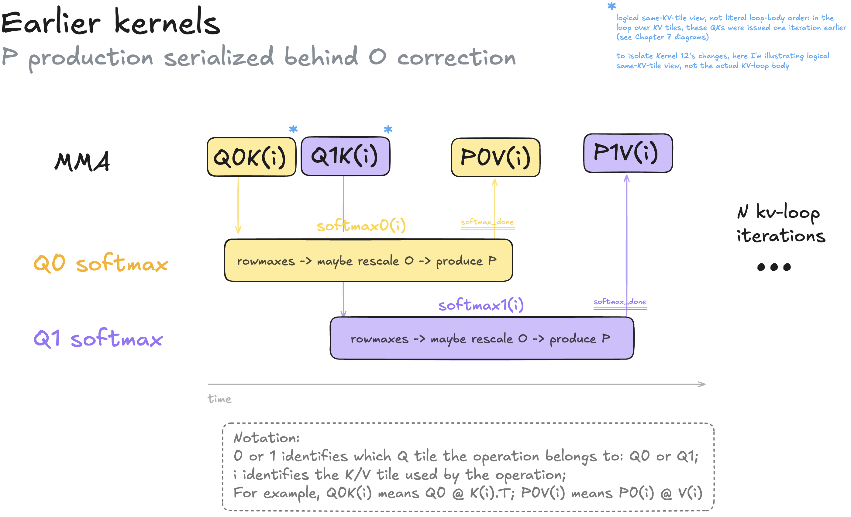
In earlier kernels, the same row warps:
- compute the current tile rowmax and the O-rescale factors;
- rescale O, if the new tile rowmax exceeds the running rowmax by the threshold (see kernel 11);
- subtract the rowmaxes from S and exponentiate to produce P.
So (2) delays completion of the row warp’s work (1-3). So O correction and P production are serialized in the same row warps.
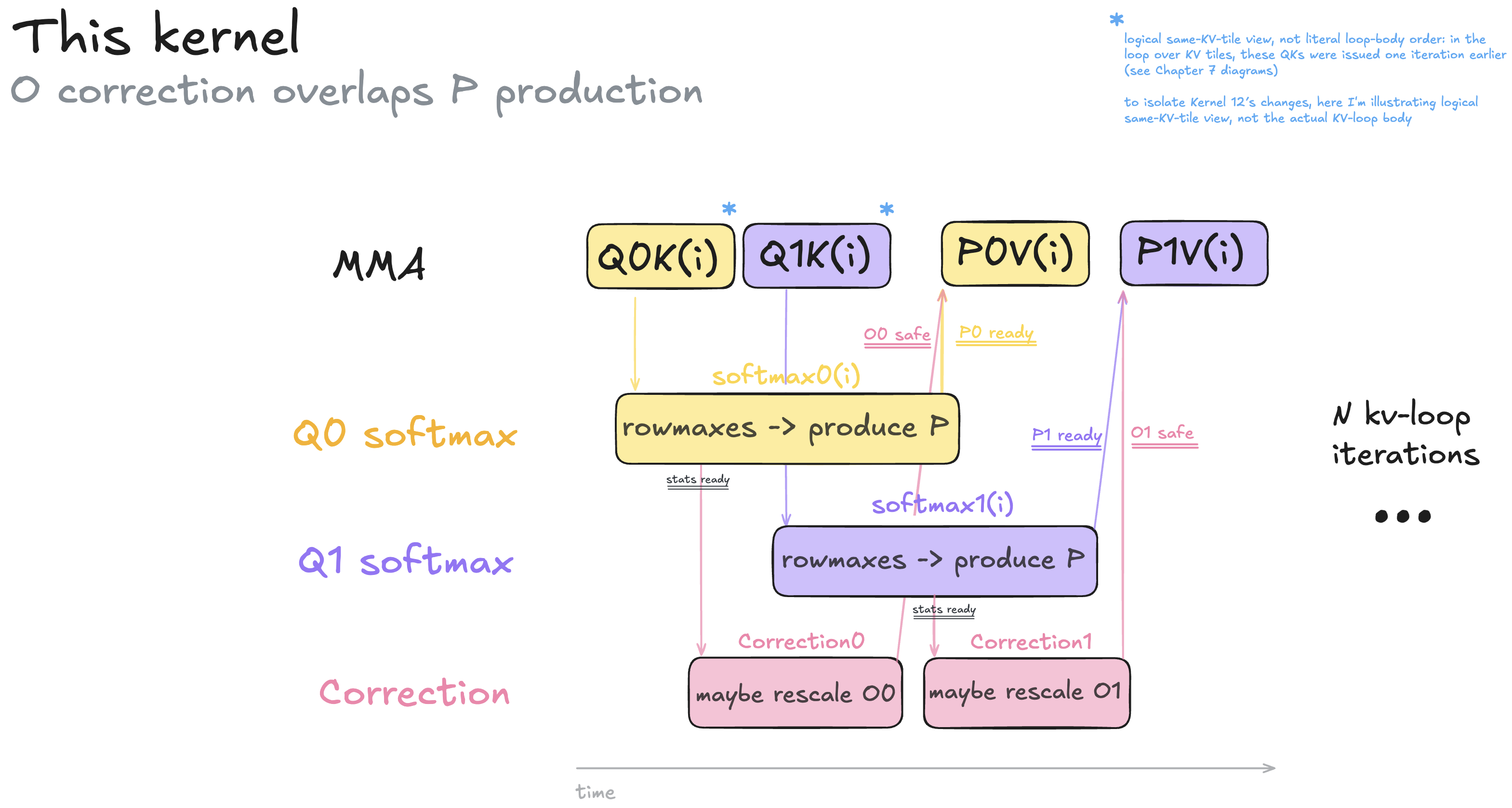
The O-rescaling (2) does not depend on computing the unnormalized-P (3), so we can move O-rescaling to separate warps which can do this work in parallel to our row warps computing the unnormalized-P (3). Therefore reducing the main bottleneck: P production (removes O correction from in front of P production, allowing the two branches to overlap). The row warps are mostly doing the softmax work now, so I’ll call them “softmax warps” from now on.
PV still requires both things to be true: P ready and O-safe, for each Q stage, these are combined into p_ready_o_safe barrier, so PV mma waits on the barrier that has 8 arrivals: 4 from softmax warps (which indicates P ready) and 4 from correction warps (which indicate O-safe). So the slowest of the two branches delays PV.
Note I deliberaly say o-safe and not o-rescaled, becuase as per our optimizations in Chapter 11, sometime we skip O rescale (so we do not always rescale O).
The softmax warps still compute the rescale factors, write the rescale factors to SMEM and signal stats_ready, and then continue producing P. The correction warps then wait for that signal, read those factors, decide whether to rebase O (if any published scale is not 1), and if so, rescale O.
The softmax warps still compute the rescale factors (as oppose to letting rescale warps do that) because the softmax warps already have the old running rowmax and the new tile rowmax in registers. Otherwise, we’d need to send that state to the correction warps and repeat the rebase logic there. So, softmax sends only one final scale value per row, and correction simply applies it to O.
The same four correction warps are shared across Q0 and Q1. For each Q stage, they read the per-row scale published by the softmax warps and use it to rescale that stage’s O tile.
KERNEL CHECKPOINT
See 12_split_correction_from_softmax.cu and diff it against Kernel 11.
Now, familiarize yourself with the code.
Performance so far
| Kernel | Change | 4k | 8k | 16k |
|---|---|---|---|---|
| 1 | Baseline | 14.2% | 14.1% | 13.7% |
| 2 | P in TMEM | 15.1% | 15.0% | 15.0% |
| 3 | Swizzling | 25.9% | 25.9% | 26.2% |
| 4 | Warp specialization | 26.6% | 26.4% | 26.5% |
| 5 | Two Q tiles | 40.5% | 40.3% | 41.3% |
| 6 | Load pipeline | 48.6% | 48.6% | 48.4% |
| 7 | Compute pipeline | 58.2% | 58.5% | 58.0% |
| 8 | Hardware exp2 | 64.1% | 64.1% | 63.8% |
| 9 | Software exp2 | 69.3% | 70.1% | 70.6% |
| 10 | Register caching | 72.9% | 73.7% | 73.6% |
| 11 | Skip O rescale | 81.7% | 83.0% | 83.3% |
| 12 | Split correction | 84.9% | 85.8% | 86.3% |
Chapter 13 – Early PV
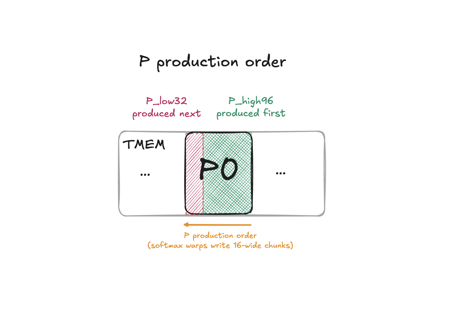
Remember P is produced right to left (written from the high end of its TMEM region towards the low end), as a consequence of our earlier optimizations (see kernel 10). So the right side of P becomes ready earlier than the entire P (by the time green box is produced, red box is not produced yet).
Kernel 13 exploits that P production order, once the
high96 P region is produced and old O is safe, a part of PV MMA can begin.
The idea is to avoid blocking PV until the entire P is ready, and instead:
do p_high96 @ V_slice1 first;
followed by P_low32 @ V_slice2 later (when P_low32 is produced).
This relies on the fact that by the time we start producing P chunks, we have already computed rowmaxes for the entire S tile, so the the running rowmax/reference is fixed, so later producing P_low32 cannot change the rowmax, and therefore cannot change already-produced P_high96.
The fact that P split visually mirrors one of our earlier optimizations from kernel 10, namely the S register caching split (both are split 32/96) is not a fundamental requirement. These two are largely orthogonal optimizations, that happen to align in our implementation.19
Note I omitted P1 (ie P of the 2nd Q stage) from the diagram cos the logic there is identical.
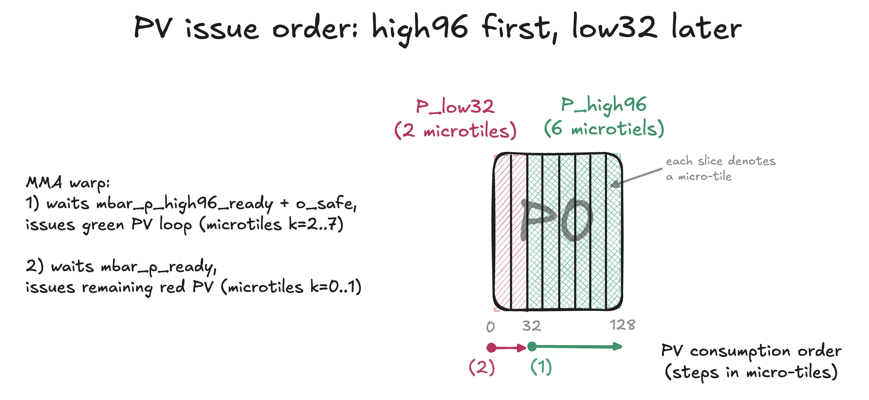
After the first barrier releases, all p_high96 is ready (ie all 6 high96 microtiles are ready, and O is safe). Once the complete high96 P region has been published, MMA does not need to consume its microtiles in the same order that the softmax warps produced them. We could have equivalently issued k=7..2; this would not meaningfully change numerics20. I kept the k=2..7 PV microtile traversal order because incrementing the corresponding V SMEM descriptor looked cleaner (so this is not a fundamental decision).
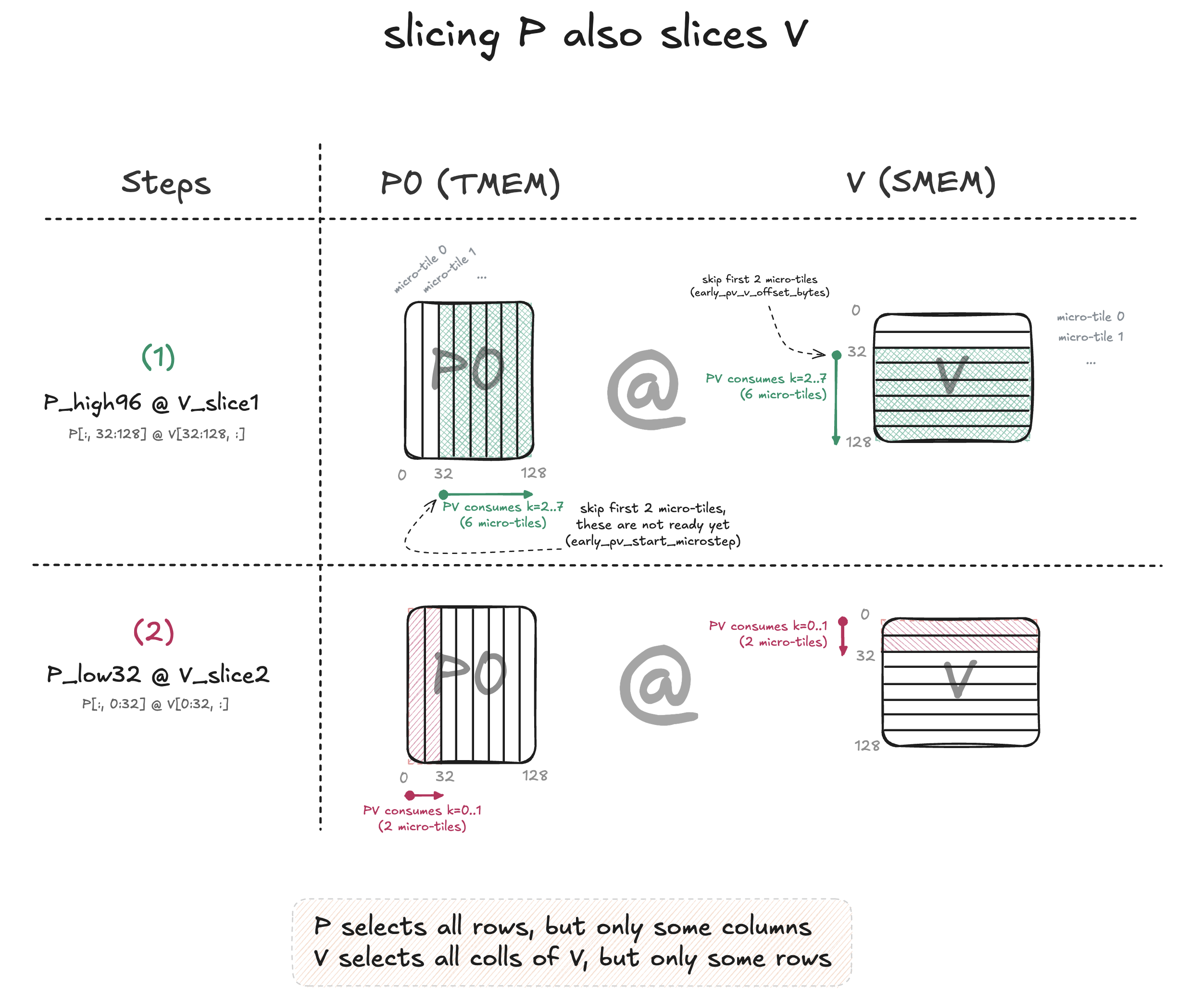
When doing the matmul with p_high96, we also need to select corresponding V slice (ie offset P’s micro-tile address and V’s descriptor by 2 microtiles). Green part of the diagram.
Later, once the softmax warps produced P_low32 and signaled that full P is ready, we matmul the remaining 2 micro-tiles (the ones we skipped earlier), P_low32 @ V_slice2. Red part of the diagram.
Both partial matmuls accumulate into the same O tile. We are only splitting P and V along the reduction axis, each into 2 chunks, together they still compute the original full P@V.
KERNEL CHECKPOINT
See 13_early_pv_96_32.cu and diff it against Kernel 12.
Now, familiarize yourself with the code.
Performance so far
| Kernel | Change | 4k | 8k | 16k |
|---|---|---|---|---|
| 1 | Baseline | 14.2% | 14.1% | 13.7% |
| 2 | P in TMEM | 15.1% | 15.0% | 15.0% |
| 3 | Swizzling | 25.9% | 25.9% | 26.2% |
| 4 | Warp specialization | 26.6% | 26.4% | 26.5% |
| 5 | Two Q tiles | 40.5% | 40.3% | 41.3% |
| 6 | Load pipeline | 48.6% | 48.6% | 48.4% |
| 7 | Compute pipeline | 58.2% | 58.5% | 58.0% |
| 8 | Hardware exp2 | 64.1% | 64.1% | 63.8% |
| 9 | Software exp2 | 69.3% | 70.1% | 70.6% |
| 10 | Register caching | 72.9% | 73.7% | 73.6% |
| 11 | Skip O rescale | 81.7% | 83.0% | 83.3% |
| 12 | Split correction | 84.9% | 85.8% | 86.3% |
| 13 | Early PV | 87.2% | 88.1% | 88.4% |
Part IV — Persistent Kernels
Chapter 14 – Persistent
Our kernels have at most one resident CTA per SM (each CTA consumes enough resources that only one can fit on an SM at a time), B200 GPU has 148 SMs, so at any given time we have up to 148 CTAs working. Since our Chapter 5 optimizations, each CTA independently consumes 2Q tiles, loop over all KV tiles, and produces 2 Output tiles.
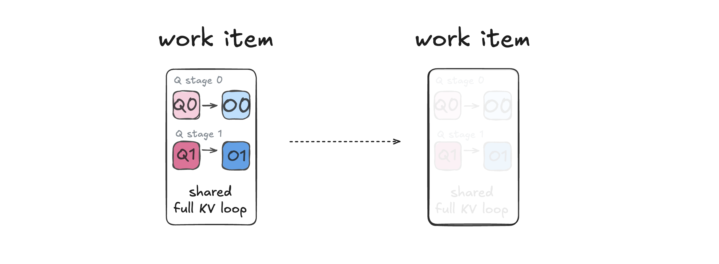
Let’s call this a “work item” and abstract this visually, like so, and our later diagram will illustrate on the granularity of work items. Our next optimization changes the lifetime around the attention body, not the body itself. So we can safely abstract it away.
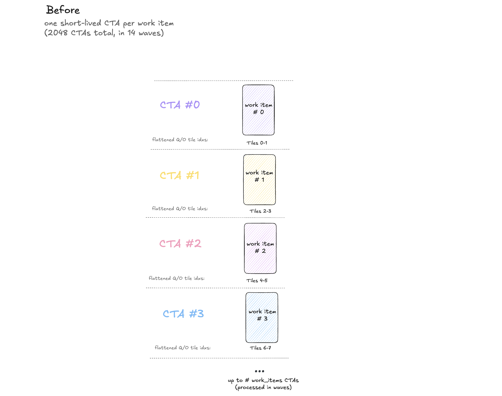
For our kernels so far, if num work items > num SMs (so there’s not enough SMs to process all our work_items at once), each SM cycles through multiple CTAs sequentially: one CTA finishes it’s work item and gets de-scheduled, another new CTA (processing a different work item) gets scheduled in its place.
These are “waves” of work.
We can compute the number of waves, by dividing total work count by the amount of work each CTA does:
For input shape SEQ_LEN=4096, for a single batch and head, and given our square tile sizes of 128,
Q and O have 4096/128=32 tiles, and because each CTA processes 2 tiles, 32/2=16 there’s only 16 work items.
So,
16 work items per batch-head
8 batches * 16 heads * 16 = 2048 total work items
For a different input shape of SEQ_LEN=16384, for a single batch, head, and given our squre tile sizes of 128,
Q and O have 16384/128=128 tiles, each CTA processes 2 tiles, so 128/2=64 there’s only 64 work items.
64 work items per batch-head
2 batches * 16 heads * 64 = 2048 total work items
So, for the 3 shapes we benchmark our kernels on,
2048 separate CTAs are launched, about 148 can be resident at once,
therefore they execute in roughly 14 CTA waves – ceil(2048 / 148 SMs) = 14 waves.
These are typically called waves. CUDA does not wait for all 148 CTAs in one wave to finish simultaneously. As soon as one CTA finishes, another waiting CTA may become resident on the freed SM, so the CTAs can drift relative to one another.
So, each SM processes roughly 14 separate CTAs sequentially: one CTA finishes, its resources are released, another CTA becomes resident. But each one of these 14 repetitions incurs the same cost: TMEM alloc/dealloc, CTA-lifetime state (setup, pointer offsets), barrier init, CTA scheduling, etc.
Fixed CTA overhead matters more at shorter SEQ_LEN
This “repeat 14 times” is the same for both 4k and 16k shapes. All 3 shapes we benchmark on (from the FA4 paper) each of them happens to have 2,048 work items (so, same fixed costs of 14 waves).
But, the KV loop grows from 32 iterations at 4K to 128 iterations at 16K, so each wave contains 4X more useful work at 16K:
KV-loop iterations = len_kv / BLOCK_N = 4096 / 128 = 32
KV-loop iterations = len_kv / BLOCK_N = 16384 / 128 = 128
So, same number of output work_items; different amount of hot-loop work inside each work_item. Thus the fixed overhead matters more for smaller-SEQ_LEN shapes: they still pay the same setup cost 14 times, but each KV loop is shorter. So, compared with longer loop lengths, the setup cost is proportionally larger for smaller SEQ_LEN shapes. Therefore, all the fixed per-CTA costs mentioned earlier take up larger part of the runtime for the shorter 4K work items.
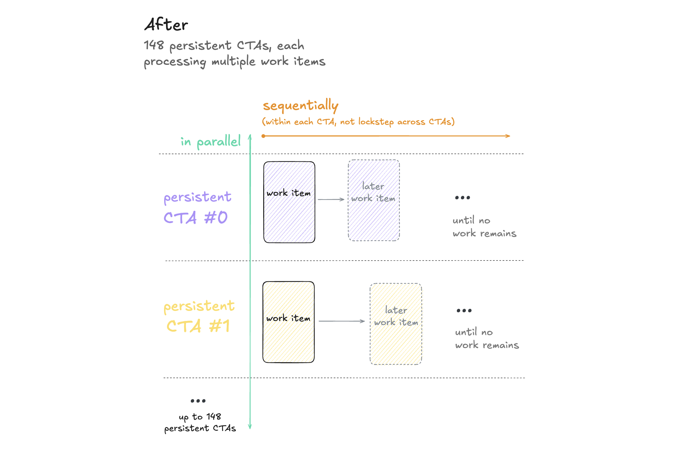
If instead, we give each CTA more work than a single work item, we can pay that cta-setup cost once but amortize it among multiple work items. And ideally the more we can amortize the better. To amortize the setup cost as much as possible, we keep each CTA alive and let it process its own sequence of 14 work items.
Note we cannot amortize: 2Q loads, KV traversal, output store, work-ID and pointer calculations. Because these legitimately differ per output work-item, even if we let one CTA process multiple work-items it still needs to re-do all these for each of the work-items it computes.
CTAs do not execute in lockstep, which is why their arrows have different lengths in the figure. So the completion of work items in one CTA can drift relative to other CTA’s progression.
Reusing barriers across work items
In earlier kernels, barriers were initialized once when the CTA started and were used for that CTA’ lifetime. Kernel 14 keeps barriers work for multiple work_items.
My first naive implementation stopped all warps between work items, waited until everything had finished, then invalidated and reinitialized the barriers before starting the next work item. That invalidation step is required by PTX, calling mbarrier.init on a barrier that is still valid is undefined. So before reinitializing, we must first make sure no warp can still be using it. It’s correct, but it creates a hard stop between work items. Every warp waits for the slowest one, all work fully drains, and only then CTA can begin its next work item.
To avoid repeated barrier init and invalidation at each of 14 work_item boundaries,
kernel 14 instead initializes all barriers once when the CTA starts,
and keeps cycling through the barrier phases as the CTA moves from one work item to the next.
The old work_done sync (where every warp waited for the slowest one and the current work fully drained)
made that barrier re-init safe, and conservatively prevented any buffer from being reused until the entire work item drained.
Kernel 14 uses the existing K/V recycle handoffs across work-item boundaries and adds q_free for Q SMEM.
Together with keeping the barriers initialized, this makes the all-warp work_done sync unnecessary.
So each buffer is released after its actual final consumer for a given work_item:
Q SMEM:
    final QK reads Q(i)
    -> q_free
    -> load Q(i+1)

K/V ring:
    final QK reads K stage
    -> refill K stage

    final PV reads V stage
    -> refill V stage
So, there is no single point where work_item(i) ends and work_item(i+1) begins. While softmax warps are still normalizing and writing O(i), load warp can begin loading next Q/K/V tiles. Once Q and K are ready, MMA warp can begin QK(i+1).
So Kernel 14 adds both persistent CTA lifetime and cross-work pipelining.
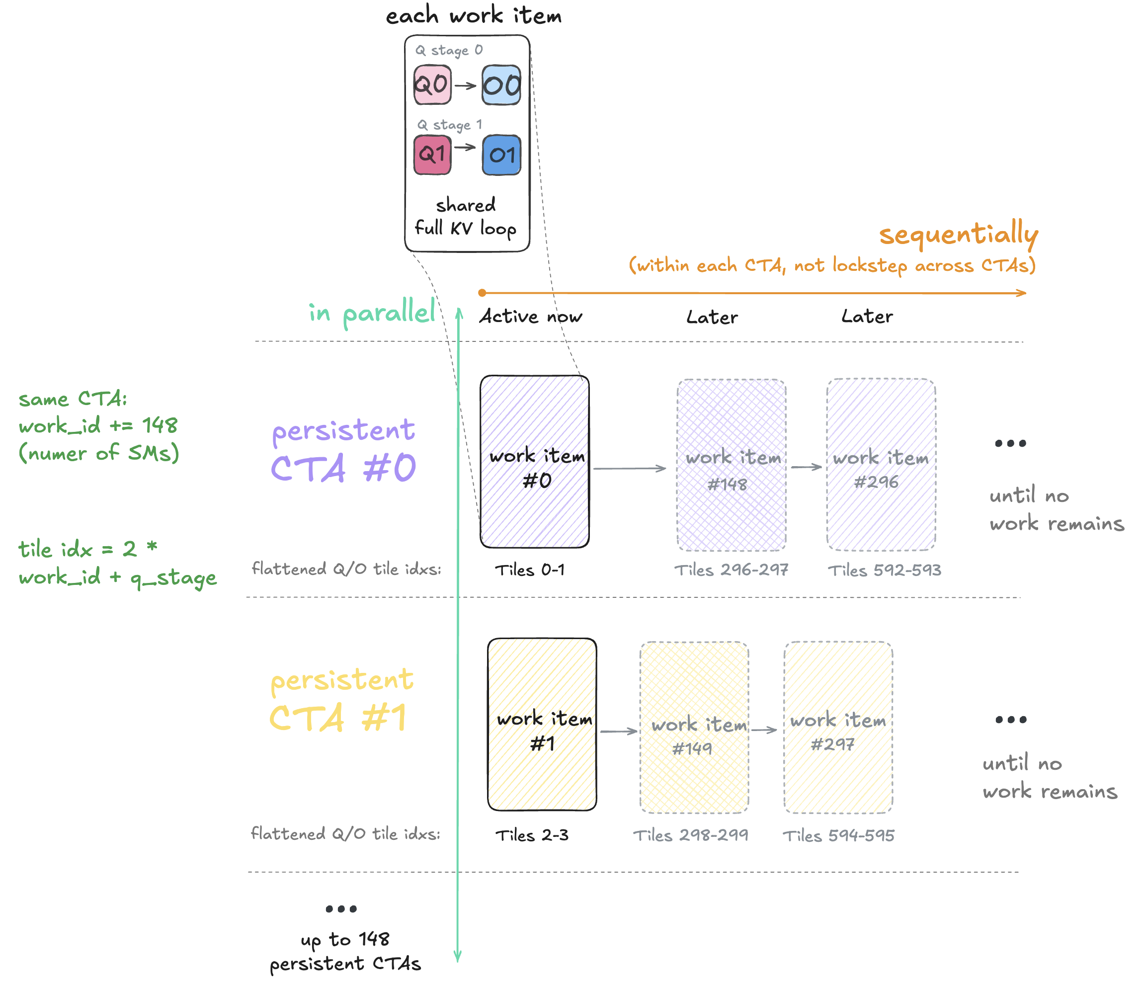
In kernel 14, each persistent CTA does not process consecutive work IDs (as illustrated in the drawing).
In code, this is just work_id += gridDim.x; // 148 CTAs
This static grid-stride assignment gives every work item to one of the 148 persistent CTAs.
Each work item covers two consecutive Q/O tiles.
So when a CTA advances by 148 work items, its tile indices advance by 296 (CTA 0 handles tiles 0–1, then 296–297, then 592–593).
I also tried assigning each CTA a consecutive range of work items. The strided assignment explained above performed better overall, though the results were shape-dependent and I haven’t tried to isolate exactly why. My guess is that shared-L2 K/V reuse helps when CTAs process different Q pairs from the same batch-head close together in time.
The figure shows which work items each CTA owns, not hard execution boundaries. As explained above, different warp roles can still overlap the end of one work item with the beginning of the next.
KERNEL CHECKPOINT
See 14_persistent.cu and diff it against Kernel 13.
Now, familiarize yourself with the code.
Performance so far
| Kernel | Change | 4k | 8k | 16k |
|---|---|---|---|---|
| 1 | Baseline | 14.2% | 14.1% | 13.7% |
| 2 | P in TMEM | 15.1% | 15.0% | 15.0% |
| 3 | Swizzling | 25.9% | 25.9% | 26.2% |
| 4 | Warp specialization | 26.6% | 26.4% | 26.5% |
| 5 | Two Q tiles | 40.5% | 40.3% | 41.3% |
| 6 | Load pipeline | 48.6% | 48.6% | 48.4% |
| 7 | Compute pipeline | 58.2% | 58.5% | 58.0% |
| 8 | Hardware exp2 | 64.1% | 64.1% | 63.8% |
| 9 | Software exp2 | 69.3% | 70.1% | 70.6% |
| 10 | Register caching | 72.9% | 73.7% | 73.6% |
| 11 | Skip O rescale | 81.7% | 83.0% | 83.3% |
| 12 | Split correction | 84.9% | 85.8% | 86.3% |
| 13 | Early PV | 87.2% | 88.1% | 88.4% |
| 14 | Persistent CTAs | 90.7% | 90.3% | 89.8% |
Minor Optimizations
Kernel 14 is the end of the main 14-kernel progression. The remaining four changes are smaller local optimizations, so I group them here. In the repo, I still keep these as separately numbered source checkpoints 15–18, so each change remains easy to diff. Together, they get us the last few percent of performance.
Deferred score acquisition. Reading S from TMEM previously used 16 loads with a wait after each load. Here, we use eight wider loads with no immediate waits, four independent rowmax chains, and a single deferred wait just before P overwrites that TMEM region, allowing load latency to overlap useful work. Most of the performance improvement comes from using four independent rowmax chains. Deferring the wait helps too, making the loads wider by itself had almost no effect.
Split rowsum accumulation. We already produce P in two parts: 96 columns from scores cached in registers and 32 columns from scores reread from TMEM. Instead of feeding both parts through one long rowsum dependency chain, here we accumulate cached 96 into two partial sums, use scalar sum for the reread 32, and combine them once.
Phase bitmasks. Every barrier stage only needs 0/1 phase, but storing these phases in small runtime-indexed arrays made the compiler place them in thread-local memory. Here we pack them into integer bitmasks instead, keeping them in registers and removing the spills.
TMA L2 promotion. Each TMA row fetch uses one 128-byte half of an aligned 256-byte region, and another nearby fetch soon needs the other half. We ask TMA to fetch the full 256 bytes into L2, making the neighboring half more likely to already be cached later when we need it; the kernel body itself does not change.
| After adding | 4k | 8k | 16k |
|---|---|---|---|
| Deferred score acquisition | 92.3% | 92.5% | 92.0% |
| Split rowsum accumulation | 93.4% | 93.7% | 93.7% |
| Phase bitmasks | 93.7% | 94.0% | 94.1% |
| TMA L2 promotion | 94.4% | 94.4% | 94.1% |
Capstone Project – Generate Videos!
Now let’s use the attention kernel we just built for something cool: generating videos. I highly recommend doing it; you will get a kick out of seeing the kernel you understand generate beautiful videos for you.
The capstone project contains the integration of our final kernel from the article (a dense BF16 attention kernel for NVIDIA B200) into the LTX-2.3 video-generation model.
To generate each video, the model will call our attention kernel 1,056 times.
You’ll need about $7 for hour of B200 compute, depending on your cloud provider. It’s enough time to set up the repo, download the weights, and generate multiple videos.
A 10.4-second video (249 frames) takes about 41 seconds to generate on B200. Runtime depends on the complete model architecture, not only on our kernel.
Don’t bother reading the video-model integration code. Your time is better spent understanding the kernel itself and its optimizations, which I already explained in this article. The capstone code simply integrates our kernel into a video-generation model and runs it.
Basically:
- Rent the compute, SSH into the machine, clone the repository, and enter
b200-attention/capstone-project. - Follow the setup and generation instructions.
- Get a kick out of seeing the near-SOTA kernel you understand generate beautiful videos for you.
The last one is the main requirement o_0.
The Graveyard 🪦 … and Some Hope ✨
Sooo… I’ve been on this problem of understanding and trying to improve over FA4 for some time.
I haven’t just tried to explain the kernel, but also developed probably tens and tens of my own new and, what seemed to me, exciting optimization ideas (not counting thousands of other ideas agents separately tried).
Improving over such heavily optimized kernel is hard. Surprise surprise :)
A couple did appear to potentially work though, but I decided to pause and finish this article before continuing my research.
I plan to share different families of my own ideas I tried, and post mortem and the learnings from there, in its own follow-up post. I’m deliberately not covering any of them here yet, until I do some more research.
Stay in touch for more ML sys
All kernels and the capstone project are available in the B200 Attention repository.
Video of my walkthrough the code is coming.
I’m also releasing a free e-book soon.
More ML systems articles, videos, and code are coming.Follow: X · LinkedIn · YouTube · GitHub
Appendix
Citation
@misc{elistratov2026b200attention,
  author       = {Elistratov, Iaroslav},
  title        = {{B200 Attention} Explained: From Scratch to Near-{SOTA}
                  in 60 Diagrams ({CUDA}/{PTX})},
  year         = {2026},
  howpublished = {\url{https://iaroslavelistratov.github.io/b200-attention/}}
}
Benchmark Calibration
FA4 is timed on contiguous BSHD, while my kernels timed on contiguous BHLD. Both receive inputs already stored in the layout they expect, so neither timing includes input-layout conversion. A direct-BSHD variant of the final kernel is provided separately. It consumes and produces contiguous BSHD without conversion copies and reaches 92.1–92.7% of same-run stock FA4.
Actually I also tried on beta29 but it’s perf was like 19% worse in my tests see discussion. So I’m sticking with the earlier version, which is faster in my tests, to avoid making my kernels look better simply because the FA4 baseline got slower due to a toolchain issue.
Official stock FA4 beta4 (CuTe DSL) against the paper numbers:
| Calibration | 4k | 8k | 16k |
|---|---|---|---|
| FA4 paper TFLOPS | 1532 | 1579 | 1601 |
| Measured stock FA4 TFLOPS | 1484 | 1528 | 1554 |
| Measured stock FA4 / paper | 96.9% | 96.8% | 97.1% |
This calibration uses 342 B200 invocations. Taking the median stock-FA4 result for each shape. On the B200s I used, even stock official FA4 itself reaches only around 97% (of their TFLOPs reported in the paper). So I mainly compare my kernels against FA4 measured in the same run (as opposed to comparing to the paper numbers).
Benchmark harness and instructions to reproduce.
How Software exp2 Works
Optional background for Chapter 9 – Software Approximations.
After Kernel 8, our exponent input is already in base-2 units, and we compute exp2(x).
Mathematically, exp2(x) = 2^x.
So we want to compute some portion of 2^x with ALUs.
We split x into its integer part and fractional part,
raise 2 to each part separately, and then multiply the two results.
Mathematically 2^(a+b) = 2^a * 2^b, so it’s equivalent to computing 2^x directly.
integer_part = floor(x)
// always between zero and one
// by our definition above
fractional_part = x - integer_part

2^x = 2^integer_part * 2^fractional_part
For example:
x                   = -3.25
integer_part        = -4
fractional_part     = 0.75
That split on the integer_part is convenient because FP32 already has a base-2 exponent
field. So, we can apply 2^integer_part by adjusting the exponent bits of the polynomial result.
But we cannot compute 2^fractional_part as conveniently as
the 2^integer_part because FP32’s exponent field can move only in whole steps
(we can move it by -4, but not by 0.75 of a step).
So we use a different method to raise 2 to the fractional_part: approximate it with a polynomial.
Because fractional_part is always between zero and one (as by our definition),
we only need to approximate one small section of the 2^x curve where x is in [0, 1).
So the exponent bits handle 2^integer_part, while the
polynomial handles 2^fractional_part.
We approximate that curve with a cubic polynomial:
2^fractional_part
    ~= 1
    + c1 * fractional_part
    + c2 * fractional_part^2
    + c3 * fractional_part^3
We can think of this polynomial as weighted blend of progressively more curved shapes. A line is too simple, while a quadratic is still not accurate enough. A cubic is flexible enough while remaining cheap to evaluate:
1                    constant, flat component
fractional_part      straight-line component
fractional_part^2    quadratic curve
fractional_part^3    cubic curve
The coefficients c1, c2, and c3 control how strongly each component contributes. They are not simply sampled values from the exponential curve. They were selected ofline to fit that curve (so that the weighted curve stays close to 2^fractional_part, on the interval between zero and one).
A small optimization we use here.
Naive implementation would first compute
fractional_part**2 and fractional_part**3,
then multiply each term by its coefficient and add everything together.
But explicitly constructing those powers costs two extra multiplications.
Instead, we keep feeding the result of one multiply-add into the
next one. So the whole cubic takes only 3 FMA instructions.
2^f ~= ((c3*f + c2)*f + c1)*f + 1
Back to Chapter 9 – Software Approximations
Acknowledgments
Thanks to the FlashAttention-4 authors, their paper and open-source CuTe DSL kernel. Thanks to CUTLASS and CuTe DSL teams, and everyone who contributed to CUTLASS Blackwell FMHA example and CuTe DSL Blackwell FMHA example.
These blogs directly inspired me to try similar format but for a different kernel:
Thien Tran: your Matmul blog is truly amazing! Highly recommend to everyone.
Modular team: Matrix Multiplication on Blackwell B200
Aleksa Gordić Anatomy of high performance Matmul kernels
Mark Saroufim: thank you for building GPU MODE and its community.
These are some of the people who inspired me to do DL and ML sys for the last 7 years.
Philippe Tillet: our chat about my earlier project inspired me a lot. I’m deeply grateful.
Edward Yang: you made me love ML sys. Few years ago, I found your PyTorch internals blog and liked it oh so much, and the torch dev podcast I’ve been listening for like 4 years.
Horace He: I appreciate our chat and your honest feedback about my earlier project; I enjoy your work Thonk From First Principles, Building ML Sys for a Trillion Trillion FLOPs. I hope we get to see more blogs from you someday, I’m sure it will be a banger.
Aleksa Gordić: I still remember your GNN project and the code you open sourced… it’s been like 6 years … oh time flies. Your matmul blog I cite above is also great.
Alexander Amini: Your MIT 6.S191 lectures kick-started my programming career.
Justin Johnson: your Michigan lectures are phenomenal.
Yannic Kilcher: 7 years ago, your videos made me love DL.
Wen-mei Hwu and coauthors, PMPP book: GPU programming starts here.
PyTorch Team: thank you for releasing Composability Syncs, I’ve enjoyed them over the years.
Do not watch random “learn CUDA” videos on YouTube. Either (1) watch the first 5 videos in this playlist. Don’t worry that these videos are old, they teach GPU-programming fundamentals that still apply today. Or (2) read the first few chapters of the Programming Massively Parallel Processors (PMPP) book. ↩︎
Hopper added TMA (separate hardware unit) which is more restricted than the ldgsts – which in turn, can be thought of as generalized gather instructions, ie each thread in a warp can compute a different offset in to the memory, which for each offset takes registers to hold the offset calculations and additional instructions (to load each thread’s element independently) – so they made a more restricted alternative to ldgsts. This saves the per-thread address-calculation instructions and the registers needed to hold these addresses. MMA already supports only a limited set of structured SMEM layouts, so giving up arbitrary per-thread addressing is not much of a restriction here. ↩︎
These micro-tile shapes come from PTX docs Table 39, which defines MMA shapes as
MxNxK, with A shapeM,K, B shapeK,N, D shapeM,N:↩︎// These numbers count BF16 elements, not bytes. For .kind::f16, no .ws, cta_group = 1, dense: - 64xNxK - 128xNxK - N = {8, 16, 24, ... 256} - K = 16A small, optional, derivation of where the (8,8) atoms shape comes from: PTX defines atom shapes in 128-bit units, not in BF16 elements. For K-major with no swizzling, PTX Table 53 defines one atom as
8×1(eight rows with one 128-bit chunk per row). Since one 128-bit chunk contains 8 BF16 values, the atom shape is (8,8) BF16 elements. ↩︎These are “unnormalized” probabilities, because in the online softmax formualtion the final division by the sum of the exponentiated values happens later, after the kv-for-loop, ie after traverals of the KV tiles. So untill we divided by the sum of the exponentiated values, this is not technically probabilities (P), but rather unnormalized probabilities. Sometimes for brevity I’ll refer to it as P, just keep in mind this is the unnormalized P. This is a minor detail, not Blackwell specific and not worth focusing on. ↩︎
tcgen05.ldsupports loading wider chunks e.g. 32 columns, not only 8 as we do here. There’s a tradeoff though as it would require less iterations along the TMEM columns but more regs to hold the wider chunks. For now I somehwat arbitrarily picked width 8. ↩︎Because P re-uses S TMEM buffer, the next QK cannot reuse that S/P slot until PV consumes P. P is produced from S, so each S region becomes dead soon after. The rest of our lineage still reaches near-SOTA perf while keeping this S/P coupling. By contrast, K is already dead after QK, while P must remain alive until PV, which is a much longer time window. ↩︎
We could load the 16 FP32 scores with one tcgen05.ld.x16 and still write the packed P with one tcgen05.st.x8. I use two ld.x8 calls only to reuse the existing width-8 load helper. ↩︎
The reason why we store P in the lower half of S and not in the upper half is not accidental: if we were to instead write P into upper half of S then we’d be overwriting unread S values, unless we change the loop over TMEM to traverse from right to left. ↩︎
NVIDIA docs tells us to expand 128b along the leading dim (based on the selected majorness). But for the
(8,8)atom shapes which the table specifies, they don’t say which of the dims, in their convention, is M/N and which one is K. So this next part is my inference from the figures. They draw M/N vertically and K horizontally. So, I read their atom shapes as (M/N, K). ↩︎Note I call them “row warps” and not softmax warps, because they don’t only compute online-softmax but also do O rescaling. ↩︎
Incidentally, that’s one of the main reasons why we use 2Q stages and not, for example, 3Q stages. Hypothetically, it seems if we let one CTA process even more Q tiles, the K/V tile SMEM loads would be amortized even more, but we’re already at TMEM limit so we have no TMEM to directly store S/P/O for the 3rd Q-tile. I did try workarounds like trying to reduce S lifetime as much as possible – by for example writing S to SMEM right after matmuls are done, and producing its P in SMEM also, thus letting the subsequent PV consume it from SMEM directly – this way the TMEM would be free for longer, potentially allowing more Q stages. But juggling data in and out of TMEM caused more overhead than the benefit of the K/V re-use introduced by 3Q tiles. ↩︎
that is, there isn’t enough TMEM for processing 2Q tiles of work for kv-loop iteration, and simultaneously processing some matmuls for iteration i+1, because these matmuls will also need to reserve TMEM and we’re already at capacity (we’re using all 512 TMEM columns) ↩︎
This is somewhat stricter than needed, K is dead after Q1K so we could re-use without waiting for P1V. But in kernel 5, the producer (load warps) still waits until P1V(i) because this kernel still recycles the K and V storage as one pair, and V remains live until that final PV. We will improve this in the later kernels. ↩︎
Three stages of complete K/V pairs would require six tile-sized KV slots. Together with Q0 and Q1, that would require 256 KiB of SMEM, which exceeds SM’ SMEM 227 KiB budget. ↩︎
Kernel 6 already has a multi-stage K/V load pipeline, so K(i+1) must be resident in another SMEM buffer, while V(i) remains available for P1V(i). ↩︎
the instruction is
ex2.approx.ftz.f32, FTZ means turn values smaller than FP32’s regular full-precision range directly into zero. Which is the additional source of approximations (in addition to hardware computing ex2.approx itself approximately). Every flushed weight is below 2^-126. ↩︎I guess I got so used to seeing rebasing after each tile in online softmax kernels, that it didn’t occur to me to question this. Untill of course, I saw FA4 source. ↩︎
There are two distinct 96/32 choices here. Kernel 10 uses 96/32 for S caching: cache high96 in regs, reread low32 from TMEM. Kernel 13 uses 96/32 for P publication: high96, start PV, then publish low32. These optimization are standalone implementaions, that don’t fundamentally require each other. Early PV itself doesn’t require the 96/32 S-caching. Mathematically, we could have published P after 16, 32, 48, 64, or 80 columns. This implementation chooses 96/32, but could have been other ratio. I tried other early_PV splits like 64/64 and others, they performed worse. ↩︎
Apart the small rounding differences caused of floating point non-associativity. ↩︎